How GPUs Share a Long Context During LLM Inference

When a model is too big for one GPU, inference engines split it with tensor parallelism: they cut every weight matrix into slices, give each GPU one slice, and let the GPUs add up their partial results. That takes care of the weights. But what if the weights fit, and it’s the long prompt that makes a request expensive?

Let’s say we serve GLM-5.3 on 8 GPUs, and a coding agent sends a request with 128,000 tokens of context. Two things are now expensive, and neither of them has much to do with the weights. First, the whole prompt has to go through all 78 layers before the first output token appears. Second, the model has to remember all 128,000 tokens for the rest of the request, which takes about 5.4 GB of KV cache. And tensor parallelism stores those 5.4 GB on all 8 GPUs (section 1.3 shows why).

Both costs grow with the number of tokens, so the obvious idea is to split the tokens across the GPUs, which is called context parallelism. If we read through the SGLang source code, though, we find that this one idea shows up as two separate features that share almost no code. One of them splits the prompt during prefill, and the other one splits the KV cache during decoding. So, why does one idea need two implementations?

In this article, I want to build up both features from what an attention layer computes, so that it becomes clear why there are two of them and what each one costs. I won’t compare inference engines here, and I will mostly stay on a single machine with NVIDIA GPUs.

This is a follow-up to How GPUs Talk to Each Other During LLM Inference, but you don’t need to have read it. I describe the mechanisms from the SGLang source code and its pull requests, which I link as we go, and the concrete numbers are for GLM-5.3. The few measurements come from two of my own pull requests to SGLang, which I tested on 4 B300 GPUs (NVIDIA’s Blackwell generation) with 4-bit NVFP4 weights and an 8-bit FP8 KV cache.

1. Why Split by Token at All#

You probably know most of this section already if you have worked with KV caches. I would still skim it, because the rest of the article keeps coming back to two things from it: the cache entry and the two phases.

1.1 What Attention Reads#

In each layer, every token produces a query, a key, and a value. To compute the output for a token, the layer compares the token’s query with the keys of all tokens up to and including it, turns the scores into probabilities with a softmax, and sums the values, weighted by these probabilities. So, what makes attention hard to split is that a token can’t be processed by itself.

However, a token never reads the tokens after it, which means that its key and value no longer change once they are computed. Instead of computing them again for every new token, a server stores them in the KV cache, which holds one cache entry per token in every layer.

1.2 Prefill and Decoding Cost Different Things#

A server handles a request in two phases. During prefill, the server processes the whole prompt at once, so every prompt token is a query. During decoding, it generates the output one token at a time, so each step has one query. Figure 1 below shows what this means for the attention layer.

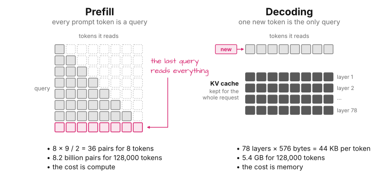
Let’s start with the left side of Figure 1. Each row is one query, and each filled square is one token that this query reads. Since a query reads everything up to itself, the squares form a triangle. For a prompt with N tokens, that’s about N²/2 pairs of a query and a key, which is 8.2 billion for our 128,000-token prompt.

Also note that the rows are not equally long. The last query reads 128,000 tokens, whereas the first one only reads itself.

On the right side of Figure 1, there is only one row. A decode step has 128,000 pairs to go through instead of 8.2 billion. However, the new token can only read the earlier tokens because their cache entries are still there, and they have to stay there for as long as the request is running.

For GLM-5.3 with an FP8 cache on Blackwell GPUs, one cache entry is a single vector of 576 one-byte numbers for all heads. Each layer keeps its own, so a single token costs 78 × 576 = 44,928 bytes, and 128,000 tokens cost the 5.4 GB. (I am using KB, MB, and GB for powers of 1,024 here.)

In short, prefill is limited by compute, and decoding is limited by memory.

1.3 What Tensor Parallelism Leaves Whole#

Now, why doesn’t tensor parallelism take care of both? After all, it distributes the attention heads across the GPUs, and for many models, that’s enough. If each attention head has its own keys and values, a GPU that holds a quarter of the heads only has to store a quarter of each cache entry.

GLM-5.3 doesn’t work this way, though. Like the DeepSeek and Kimi models, it uses Multi-Head Latent Attention (MLA), which compresses the keys and values of a token into one small latent vector that all heads read. This vector is the cache entry from section 1.2. Tensor parallelism can split the heads and the weights but not this vector, so every GPU stores and reads the same context, as Figure 2 below illustrates.

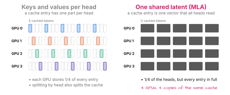
As we can see on the right side of Figure 2, splitting by head doesn’t split anything here. With 8 GPUs, our 128,000-token request takes 8 × 5.4 GB = 43 GB of GPU memory, and 7 of the 8 copies are redundant.

There is a second thing that tensor parallelism leaves whole, and it has to do with prefill. GLM-5.3 uses sparse attention (DeepSeek Sparse Attention, DSA), where a token doesn’t read all the earlier tokens. Instead, a small module called the indexer first gives every earlier token a relevance score and passes only a fixed number of the highest-scoring tokens on to the attention heads. In GLM-5.3, 21 of the 78 layers run the indexer, and the other layers reuse the selection of the layer before them. To do its scoring, the indexer keeps a small cache of its own, the index, with one index key per token.

The problem is that the indexer is not divided by head, so tensor parallelism has nothing to distribute: every GPU sees every token and computes the same scores for every query. With sparse attention, it’s the indexer that goes through the 8.2 billion pairs from section 1.2, and with 8 GPUs, it does so 8 times.

1.4 Three Collectives#

Splitting by token means that the GPUs have to exchange data, and almost every exchange in this article is one of three operations. They are called collectives because all the GPUs in a group take part, which also means that a collective is only finished once the slowest GPU is done. Figure 3 below shows what each of them does to the data on 4 GPUs.

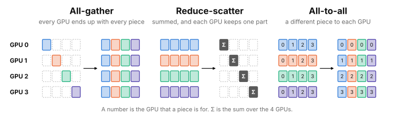
Let’s go through Figure 3 from left to right. In an all-gather, every GPU hands out the piece it has, so that every GPU ends up with all of them, and nothing is summed. In a reduce-scatter, every GPU starts with a full-sized tensor, the tensors are summed across the GPUs, and each GPU only gets its own part of the sum back. Finally, in an all-to-all, every GPU sends a different piece to each of the other GPUs, and again, nothing is summed.

1.5 Summary#

To summarize, prefill has to work through a triangle of about N²/2 pairs, and decoding has to keep one cache entry per token and layer in memory. Tensor parallelism splits the weights and the heads, but for a model like GLM-5.3, it leaves two things whole: the KV cache, because all heads read the same cache entry, and the indexer, because it runs before the heads.

For every mechanism that splits by token instead, I will ask the same three questions: what does one GPU store, what crosses between the GPUs in each attention layer, and what does it cost? For tensor parallelism, the answers are short: each GPU stores the whole cache and the whole index, what crosses is the summed attention output, and the cost is 8 copies of everything that grows with the tokens. We will collect the answers in one figure at the very end.

2. Prefill Context Parallelism#

Let’s start with prefill, since it is the easier one to picture: if the prompt has too many queries for one GPU to handle quickly, we give each GPU only a share of them.

2.1 One Forward Pass#

With C GPUs, each GPU keeps 1/C of the prompt tokens and carries them through the whole model. The attention module is where this gets interesting, because a query has to read the keys and values of all the earlier tokens, and most of those are now on other GPUs.

SGLang solves this in the most direct way. In every attention layer, each GPU first computes the keys and values for its own tokens. Then, an all-gather hands them to all the other GPUs, where they are put back into the original token order and written to the KV cache. After that, every GPU has the keys and values of the whole prompt and can run attention for its own queries, as shown in Figure 4 below. The figure also shows the feed-forward module, a Mixture-of-Experts (MoE) module in these models, which we will get to in a moment.

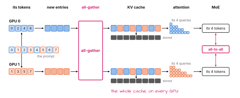
As Figure 4 shows, each GPU now runs attention for only half of the queries. And in contrast to tensor parallelism, this also applies to the indexer from section 1.3, so together the GPUs score the 8.2 billion pairs once instead of 8 times.

The attention module and the MoE module don’t have to be split the same way, since SGLang converts between the two at their boundary. So, the rest of the layer depends on the MoE module. With expert parallelism, as in Figure 4, each GPU holds different experts and sends its own tokens to them through the all-to-all that expert parallelism needs anyway. A tensor-parallel MoE module needs every token on every GPU to sum the partial results, so SGLang all-gathers the tokens before it and returns each GPU’s tokens with a reduce-scatter.

The price on the attention side is the all-gather. For GLM-5.3 on Blackwell GPUs, it carries the 576-byte entry of each token, which adds up to about 70 MB per layer over our 128,000-token prompt. (Servers feed a long prompt through in chunks, so a single all-gather only carries one chunk of this. The layers that run the indexer add a second, smaller all-gather for the index keys.) The all-gather grows linearly with the prompt, whereas the attention work that we are splitting grows quadratically, so the longer the prompt, the better this trade becomes.

Figure 4 gave GPU 0 the even tokens and GPU 1 the odd ones. Why didn’t it simply use the first and second halves?

2.2 Why Consecutive Pieces Don’t Work#

The obvious choice is to cut the prompt into C consecutive pieces and give one to each GPU.

The problem with this is the triangle from Figure 1: the GPU with the last piece has much more work to do than the GPU with the first piece. We can work out by how much. The queries of the first piece read, on average, half of their own piece. The queries of the last piece read the C − 1 pieces before them plus half of their own. That’s C − ½ against ½, so the last piece has 2C − 1 times as many pairs as the first one. With 8 GPUs, that’s a factor of 15.

This matters because the all-gather in every layer waits for the slowest GPU, so the other 7 GPUs idle about half the time. Figure 5 below shows this imbalance with a small example, next to the two layouts that SGLang uses.

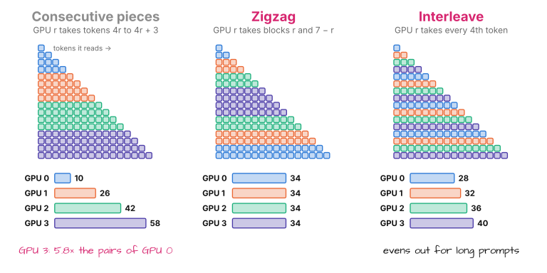
On the left side of Figure 5, GPU 3 ends up with 58 pairs and GPU 0 with 10. That’s a factor of 5.8 and not the 7 that the formula gives for 4 GPUs, because the formula is only exact for long prompts.

2.3 Zigzag#

The first layout is called zigzag, and it fixes the imbalance with a simple trick: every GPU gets some cheap tokens and some expensive ones.

To do this, zigzag cuts the prompt into 2C blocks instead of C. GPU 0 takes the first block and the last block, GPU 1 takes the second block and the second-to-last block, and so on. This is the middle panel of Figure 5.

Why does this balance out? Let’s number the blocks from 0 to 2C − 1 and count the work in units of “one block of queries reading one block of keys.” As with the pieces in the previous section, block b reads the b blocks before it plus half of itself, so it costs b + ½ units. GPU r has block r and block 2C − 1 − r, which add up to (r + ½) + (2C − 1 − r + ½) = 2C units. The r cancels out, which means that every GPU does exactly the same amount of work. Figure 6 below shows the pairing for 4 GPUs.

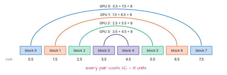
In Figure 6, the cheapest block is paired with the most expensive one, the second cheapest with the second most expensive, and so on, so every pair costs 8 units.

A regular attention kernel expects a run of consecutive queries and takes care of the triangle inside that run by itself, so all it needs to know is where the run ends. My guess is that this is the second reason why zigzag is attractive: in SGLang’s implementation, each GPU calls such a kernel once per block and passes it one number, namely where that block’s reads end.

(If the beginning of the prompt is already cached from an earlier request, only the new tokens are split, and both blocks still read the cached part.)

2.4 Interleave#

The second layout is even simpler. It hands out the tokens one at a time: token 0 goes to GPU 0, token 1 to GPU 1, and so on, and after C tokens, it starts over at GPU 0. In code, this is a single line (simplified from here):

# cp_size = C, cp_rank = this GPU's number
my_tokens = tokens.view(-1, cp_size, hidden_size)[:, cp_rank]

As we can see on the right side of Figure 5, each GPU now has queries from all over the prompt, so the load evens out without any pairing. Each query on GPU 1 still sits one position later than the corresponding query on GPU 0 and reads one more token, but with 128,000 tokens and 8 GPUs, that’s about 0.01% more work for the busiest GPU.

Why would we use zigzag at all, then? The catch is that interleave gives up the consecutive runs. Neighboring queries on a GPU are now C positions apart, and each of them reads up to a different point, which doesn’t fit the interface of a regular attention kernel.

For sparse attention, this is not a problem, because every query there comes with its own list of selected tokens anyway. I assume that’s why SGLang uses interleave for the sparse-attention models (DeepSeek-V3.2, the GLM-5 series, and DeepSeek-V4 on NVIDIA and AMD GPUs) and zigzag for models with regular attention. In fact, it rejects zigzag altogether for DeepSeek-V3.2.

SGLang didn’t invent the interleave layout. Handing out the tokens in stripes to balance this triangle was proposed in 2023 as Striped Attention, for training with very long sequences.

2.5 Summary#

To summarize in terms of our three questions, each GPU computes 1/C of the queries but still stores the whole cache. What crosses, and what it costs, are the new cache entries in one all-gather per attention layer (two where the indexer runs), plus the tokens around a tensor-parallel MoE module. Zigzag pairs an early block with a late block, which balances the work exactly, and interleave takes every C-th token, which balances it almost exactly and fits sparse attention well.

How much does this help in practice? The only number I have is a rough one, from the test notes of an earlier pull request of mine for GLM-5.2, the predecessor of GLM-5.3. There, turning on prefill context parallelism reduced the time to the first token by about half for 128,000-token prompts. The two runs didn’t use the same chunk size, though, so I wouldn’t read more into it than “it helps a lot.”

There is one thing that prefill context parallelism doesn’t do. Look at the KV cache column in Figure 4 again: after the all-gather, every GPU writes the cache entries of all the tokens to its own KV cache. So, by default, every GPU still holds the full 5.4 GB after prefill.

For prefill, that’s fine, since compute is the bottleneck there. For decoding, memory is the bottleneck, which brings us to the second feature.

3. Decode Context Parallelism#

During decoding, there is nothing left to split on the query side, because each step has only one query. What we want to split instead is the KV cache.

3.1 Storing Each Token Once#

The idea is to store the cache entry of each token on exactly one GPU instead of on all of them. Decode context parallelism does this in a round-robin fashion, as the interleave layout does with the queries. With C GPUs, it stores token p of a request on GPU p mod C, as shown in Figure 7 below.

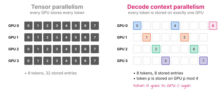
As we can see in Figure 7, each GPU now holds a quarter of the request. With 8 GPUs, our 128,000-token example takes 0.7 GB per GPU instead of 5.4 GB, and the freed memory can hold more context or more requests.

A nice property of this scheme is that the server keeps one numbering of cache positions (I will call them slots), as if there were a single cache that is C times larger. The parts that hand out cache positions and reuse cached prefixes therefore keep working as before. Only the code that reads and writes the cache translates a slot number into a GPU and a row on that GPU:

gpu = slot % C
row = slot // C

So, slot 9 on 4 GPUs is row 2 on GPU 1.

3.2 Why the Results Can’t Simply Be Added#

This creates an obvious problem, though. The new token has to read all the cached tokens, and each GPU can now only see its own share of them.

The natural thing to try is to let each GPU run attention over its own share and then add up the results. Unfortunately, this gives the wrong answer, and the reason is the softmax. A softmax divides each exponentiated score by the sum of the exponentiated scores of all the tokens it sees. If a GPU only sees a quarter of the tokens, it divides by a sum that is too small, so all of its probabilities come out too large.

This is easier to see with a small example. Let’s take 4 cached tokens on 2 GPUs, as shown in Figure 8 below.

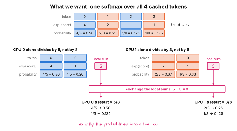
The top of Figure 8 shows what we want. The 4 tokens have the (exponentiated) scores 4, 2, 1, and 1, which add up to 8, so the probabilities are 0.50, 0.25, 0.125, and 0.125.

The middle shows what each GPU computes by itself. GPU 0 only sees tokens 0 and 2, so it divides by 5 instead of 8 and gets 0.80 and 0.20. GPU 1 divides by 3 and gets 0.67 and 0.33. Together, that’s 4 probabilities that add up to 2.

But notice that the probabilities of each GPU are not wrong in an arbitrary way: they are all too large by the same factor. GPU 0 divided by 5 where it should have divided by 8, so if we multiply its result by 5/8, we get 0.50 and 0.125, which is exactly right. For GPU 1, the factor is 3/8.

This means that all a GPU has to report in addition to its result is one number, its local sum. With the local sums of all GPUs, we know the total, and with the total, we can rescale the partial outputs and add them up.

3.3 The Log-Sum-Exp Merge#

In practice, the GPUs don’t exchange the sum itself but its logarithm, which is known as the log-sum-exp (LSE). The reason is that the sum of exponentials can easily overflow, and attention kernels already compute it in log space to avoid this.

Below is a simplified excerpt of the more readable of SGLang’s merge variants (the full version is here):

# Simplified from layers/dcp/comm.py
lses = all_gather(my_lse)                    # the LSEs of all GPUs
global_lse = torch.logsumexp(lses, dim=0)    # the log of the total

scale = torch.exp(my_lse - global_lse)       # my share of the total
out = reduce_scatter(my_out * scale)         # add up the rescaled outputs

In terms of Figure 8, scale is 5/8 for GPU 0 and 3/8 for GPU 1.

This is not an approximation: apart from the order in which floating-point numbers are added, the merged result is the same as that of a single softmax over all the tokens. The accuracy check in my pull request for GLM-5.3 agrees with this. On the 1,319 math problems of GSM8K, GLM-5.3 solves 1,283 with plain tensor parallelism and 1,279 with the cache split across 2 or 4 GPUs, which is within the noise.

3.4 One Decode Step#

There is one more complication: the weights are still split by tensor parallelism, so each GPU holds the projection weights for its own group of attention heads and can only compute the query for those heads. Let’s call such a group a head slice. (The SGLang documentation calls it a head shard.) With 4 GPUs, there are 4 head slices, and GPU 2 owns head slice 2.

Now, head slice 2 has to read all the cached tokens, but three quarters of them are stored on other GPUs. Either the cache entries have to travel to GPU 2, or the query of head slice 2 has to travel to the cache entries. Sending the entries gets more expensive the longer the context is, whereas a query always has the same size. As far as I can tell, that’s why the query is the one that travels.

This takes five steps, as illustrated in Figure 9 below.

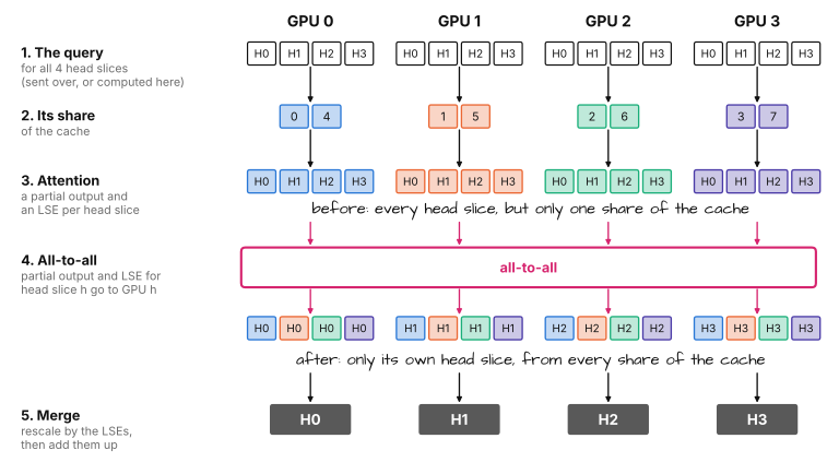
Let’s go through Figure 9 from top to bottom. First, every GPU needs the queries of all 4 head slices, not only its own (the next section shows where it gets them from). Second, it looks up the cache entries that it stores. Third, it runs attention for all 4 head slices over these entries, which gives a partial output and an LSE per head slice, each covering only a quarter of the cache.

In the fourth step, an all-to-all sends each partial output to the GPU that owns its head slice, so GPU 2 ends up with 4 partial outputs for head slice 2, one from each GPU’s share of the cache. In the fifth step, each GPU combines them with the LSE merge from section 3.3 and now holds its own head slice, computed over the whole cache. This is what it would hold with plain tensor parallelism, so nothing after the attention module has to change.

3.5 All-to-All or All-Gather plus Reduce-Scatter#

Figure 9 used a single all-to-all for the exchange. That is the newer of two ways in which SGLang runs a decode step, and what differs between them is the number of collectives per attention layer, as shown in Figure 10 below.

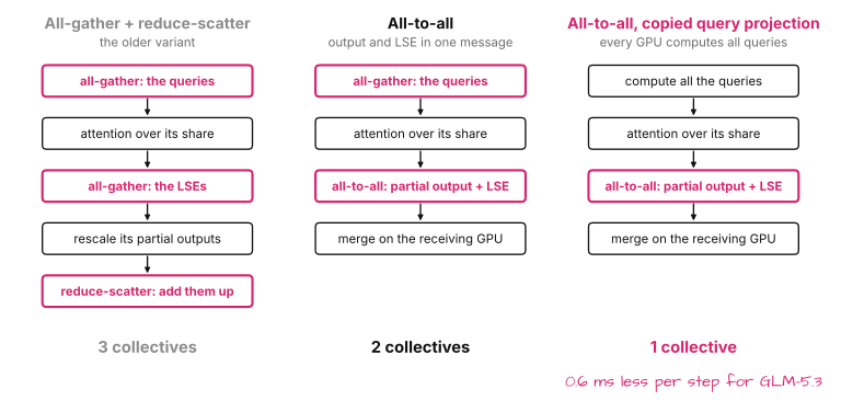
The older variant, on the left side of Figure 10, is the one from the code excerpt in section 3.3. It needs three collectives: an all-gather for the queries, an all-gather for the LSEs, and a reduce-scatter that adds up the rescaled partial outputs and gives each GPU its own head slice back. The all-to-all in the middle packs each partial output and its LSE into one message, so the receiving GPU can do the merge by itself, which leaves two collectives.

The right side removes the query all-gather as well. The queries have to travel because each GPU holds the query projection weights only for its own head slice. If every GPU keeps a full copy of these weights, which SGLang gathers once at startup, it can compute all 4 queries by itself. This costs some weight memory and matrix multiplication work, and it only applies to weights that are not quantized, but it leaves a single collective per layer. Kimi K3 and my pull request for GLM-5.3 both turn the copy on.

By the way, decode context parallelism is not SGLang’s invention either. Splitting the cache by token inside the attention module and then going back to the usual tensor-parallel or expert-parallel split for the feed-forward module was proposed as Helix Parallelism. SGLang’s roadmap also credits the copied query projection to that paper.

3.6 What It Costs#

So, what do we pay for the smaller cache? Decode context parallelism doesn’t make the attention computation any cheaper, since each GPU handles C times as many head slices but over only 1/C of the tokens, which roughly cancels out. The gain is memory, and the price, with the all-to-all, is one additional collective per attention layer, or two with gathered queries.

To get a feel for the size of this trade, here are a few numbers from my pull request, measured with a single request and 32,000 tokens of context. The server always has 4 GPUs. “Split across 2 GPUs” means 2 pairs that each hold a full copy, so every entry is still stored twice.

With plain tensor parallelism, a decode step takes 6.78 ms. With the cache split across 2 GPUs, it takes 7.61 ms, and across all 4 GPUs, 8.08 ms. In other words, a step gets 12% or 19% slower. In return, the same 4 GPUs can hold 1.8 or 3.1 times as many tokens. That’s not quite 2 and 4, and section 4 explains why.

These numbers are with the query projection copied to every GPU. Without the copy, the 2-GPU split takes 8.25 ms instead of 7.61 ms, so the 78 all-gathers for the queries cost about 0.6 ms per step.

3.7 Summary#

To summarize in terms of our three questions, each GPU stores 1/C of the cache and runs attention over its own share for all head slices. What crosses in every attention layer are the partial outputs, which give the exact result once they are rescaled with their LSEs, and also the queries unless the query projection is copied. The cost is those one or two collectives.

This mechanism is not specific to SGLang: vLLM, another inference engine, has the same feature under the same name, and the open InferenceX benchmark uses it for Kimi K3 with the cache split across 16 GPUs.

4. Sparse Attention: Copy the Index or Split It#

In section 3, I pretended that the new token reads all the cached tokens. For GLM-5.3, that’s not quite true, since the indexer from section 1.3 selects the tokens first, and it needs its index to do so. This raises a question that doesn’t come up with regular attention: if we split the KV cache across the GPUs, what do we do with the index?

4.1 Two Options#

Figure 11 below shows the two options side by side.

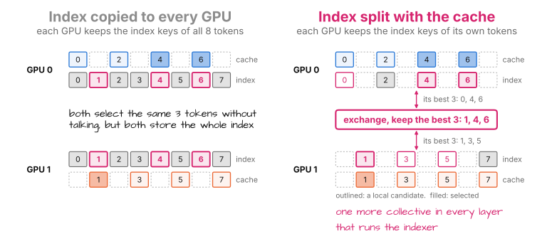
The first option, on the left side of Figure 11, is to leave the index alone, so that every GPU keeps the index keys of all the tokens. Since the indexer is not divided by head, every GPU then selects the same tokens without having to talk to the others, picks out the ones that it stores itself, and runs attention over them as in Figure 9.

The second option, on the right side of Figure 11, is to split the index along with the cache. Each GPU then only keeps the index keys of its own tokens, so it can’t know by itself which of them make it into the overall selection. In Figure 11, GPU 0 would pick tokens 0, 4, and 6 from its own half, but token 0 loses against token 1, which only GPU 1 can score. To arrive at the same selection anyway, the GPUs have to exchange their best candidates and pick the overall best from them. That’s one more collective for every layer that runs the indexer.

4.2 How Much Memory a Copied Index Costs#

The nice thing about this trade is that we can calculate the memory side. Let’s call the number of bytes that the KV cache needs per token E, and the number of bytes that the index needs per token I.

With plain tensor parallelism, each GPU spends E + I bytes per token. If we split the cache across C GPUs but copy the index, each GPU spends E/C + I. So, the number of tokens that fit grows by a factor of (E + I) / (E/C + I) instead of the full factor of C.

For GLM-5.3, E is the 44,928 bytes from section 1.2, and I is 2,772 bytes (21 layers × 132 bytes). The capacity then grows 1.89 times with 2 GPUs, 3.41 times with 4 GPUs, and 5.69 times with 8 GPUs.

At 2 GPUs, we get 95% of what a split index would give us, which means that copying costs very little. At 8 GPUs, we only get 71%, because the index, which stays the same size, has become a noticeable part of what each GPU stores. And no matter how many GPUs we add, the factor can never exceed (E + I) / I, which is 17.2. Figure 12 below shows both effects.

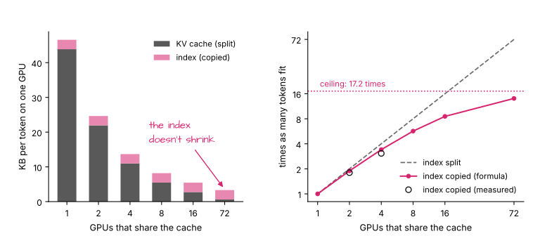
On the left side of Figure 12, the gray part of each bar shrinks with the number of GPUs, whereas the pink part stays the same size. The two are equal at C = E/I, which is 16.2 for GLM-5.3, and beyond that, a GPU stores more index than cache. The last bar is the 72 GPUs of a GB300 rack, which we will come back to in section 10. On the right side, the fixed index is why the curve for the copied index bends away from the dashed line and flattens out below the ceiling.

The two hollow markers are the 1.8 and 3.1 from section 3.6. They sit a bit below the formula’s 1.89 and 3.41, which I attribute to a few buffers that grow with the number of GPUs sharing the cache.

4.3 How Much Communication a Split Index Costs#

What about the other side of the trade? Since only 21 of the 78 layers of GLM-5.3 run the indexer, a split index adds 21 collectives to every decode step.

I don’t have a measurement for these, but we can make a rough estimate. The 78 all-gathers for the queries in section 3.6 cost about 0.6 ms per step, or 8 microseconds each. If the 21 additional collectives cost the same, they would add less than 0.2 ms on top of a step of 7.6 ms, or about 2%.

This is only an estimate, since a list of candidates doesn’t have the same size as a query, and the 8 microseconds were measured with the cache split across 2 GPUs and not across 8. But if it is about right, splitting the index at 8 GPUs would raise the capacity from 5.69 to 8 times, which is 41% more tokens for steps that are 2% slower. I think that would be worth it. At 2 GPUs, the gain would be only 6%, which probably doesn’t justify the extra code.

My pull request copies the index, and I only tested it with 2 and 4 GPUs.

4.4 Summary#

To summarize, a copied index costs memory: a GPU stores E/C + I bytes per token, with a ceiling that matters more as more GPUs share the cache. A split index costs communication: a GPU stores (E + I) / C, but each layer that runs the indexer needs one more collective for the candidates.

5. Handing the Cache from Prefill to Decoding#

Section 2 leaves the full cache on every GPU, whereas section 3 stores each entry only once, so the two features don’t fit together well. In SGLang today, they are usually not used on the same server. Instead, a common setup is a disaggregated deployment, where one server does prefill and a second server does decoding. Each server is set up for its own phase, but the first one has to send the KV cache to the second. What it sends depends on what each prefill GPU holds and on what each decode GPU wants to store, and Figure 13 below shows three cases.

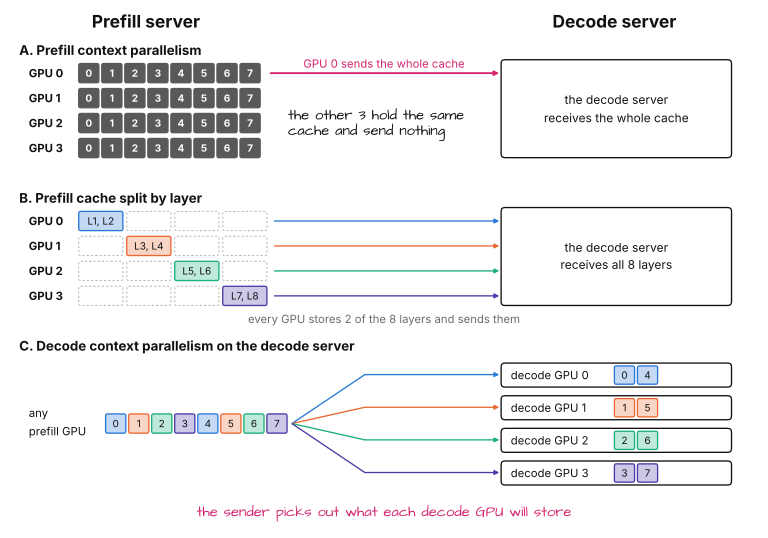
In Figure 13, case A is prefill context parallelism. Since every prefill GPU holds the whole cache after the all-gather, there is nothing to coordinate: one GPU sends its copy, and the others send nothing.

Case B gets rid of the waste in case A. A GPU needs the cache entries of a layer only while it works on that layer, so SGLang can also split the prefill cache by layer, as an option for the sparse-attention models with the interleave layout. Each GPU keeps the entries for a range of layers and holds the others only in a temporary buffer while it works on them. Every GPU then holds something different, so all of them take part in the hand-off.

InferenceX uses case B in a recipe for GLM-5.2 on H200 GPUs. Its prefill server lets all 8 GPUs share the tokens with the interleave layout and splits the cache by layer. The decode server uses DP attention, the topic of the next section.

In case C, the decode server uses decode context parallelism. The prefill server stores the cache in the usual way, but the decode server wants token p on GPU p mod C. Before sending, the prefill server therefore picks out the entries that each decode GPU will store and packs them together.

Figure 13 has no fourth case with prefill context parallelism on one side and decode context parallelism on the other, because SGLang currently rejects that pairing. A decode server that splits its cache expects a prefill server with tensor parallelism or with pipeline parallelism, where consecutive groups of layers live on different GPUs. A draft pull request aims to lift this restriction for GLM-5.3, with 8 GPUs sharing the tokens on the prefill server and 8 GPUs sharing the cache on the decode server.

6. Decode Context Parallelism or DP Attention?#

The InferenceX decode server above uses DP attention, not decode context parallelism. DP attention is the older way to avoid storing an MLA cache on every GPU. So, why do we need a second one?

6.1 Two Ways to Avoid the Copies#

DP attention (DP for data parallelism) leaves the rest of the model as it is but doesn’t split the attention module at all. Each GPU runs the complete attention module for its own share of the requests and keeps only their KV cache.

DP attention splits the requests, and decode context parallelism splits the tokens of each request. Figure 14 below shows what this means for the memory of each GPU.

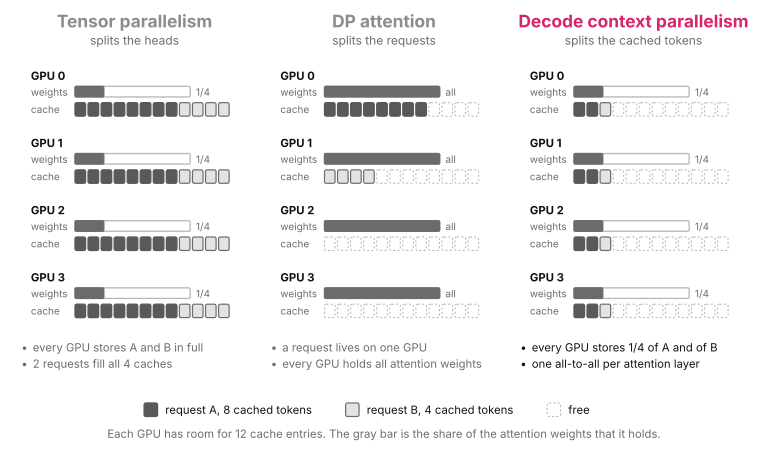
The first difference between the middle panel and the right one is where a request lives. With DP attention, a request sits in a single DP attention group (one GPU in Figure 14), so its context can’t grow beyond what that group can hold. With decode context parallelism, each request is spread over all the GPUs, so a single long request can use the memory of all of them.

The second difference is the gray bar. With DP attention, every GPU needs all of the attention weights, since it runs the complete attention module. With decode context parallelism, only the query projection may be copied. For Kimi K3, the full copy takes about 72 GB on every GPU, memory that the cache could have used, according to the SGLang post about this model.

Of course, DP attention has an advantage as well: it doesn’t need any of the collectives from Figure 9.

6.2 What the Numbers Say#

Which one is faster, then? Figure 15 below shows the throughput sweep from my pull request, with the same setup as in section 3.6.

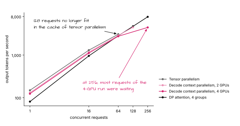
Let’s read Figure 15 from left to right. For a single request, plain tensor parallelism is the fastest with 149 tokens per second, and decode context parallelism is close behind (131 across 2 GPUs). DP attention only reaches about 80, I assume because fewer GPUs work on the attention module of a given request.

At 64 concurrent requests, all four are within 11% of the fastest. After that, two of the lines end because the requests no longer fit: tensor parallelism can’t hold 128 requests of this length, and the cache split across 2 GPUs can’t hold 256.

At 256 concurrent requests, DP attention is clearly ahead. This comparison is not quite fair, though, since the cache split across 4 GPUs couldn’t hold all 256 requests at once, and most of them were waiting in the queue.

Overall, plain tensor parallelism is the fastest of the three as long as everything fits. When a few long requests no longer fit, I would expect decode context parallelism to be the next step, because it keeps most of the per-request speed. I haven’t measured this, because the sweep doesn’t include such a request. DP attention looks like the better choice for many concurrent requests, although this sweep can’t show by how much. In terms of our three questions, DP attention stores a whole request on one GPU, nothing crosses for the attention module, and the cost is all the attention weights on every GPU.

7. The Flags in SGLang#

How do we turn all of this on? A few of SGLang’s flags are easy to misread, mostly because --tp-size is the total number of GPUs and the other flags divide it. Figure 16 below shows what four typical combinations do to the GPUs.

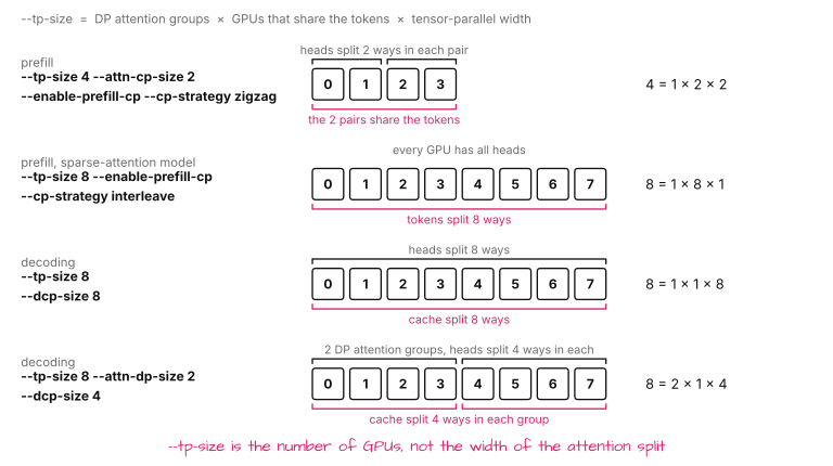
As the line at the top of Figure 16 says, the attention module divides the total three ways. --attn-dp-size sets the number of DP attention groups, --attn-cp-size sets how many GPUs share the tokens during prefill, and the rest is the tensor-parallel width. In the first row, which is an example from the SGLang documentation, 4 GPUs with --attn-cp-size 2 end up as 2 tensor-parallel pairs, with the tokens split between the pairs.

To turn on prefill context parallelism, we pass --enable-prefill-cp, and we choose the layout from section 2 with --cp-strategy zigzag or --cp-strategy interleave. Below is an example for GLM-5.2 on 8 GPUs, which corresponds to the second row of Figure 16:

sglang serve \
  --model-path zai-org/GLM-5.2-FP8 \
  --tp-size 8 \
  --enable-prefill-cp --cp-strategy interleave \
  --attention-backend dsa \
  --trust-remote-code

Note that there is no --attn-cp-size in this command. For the sparse-attention models, SGLang lets all GPUs share the tokens by default, which leaves a tensor-parallel width of 1 for the attention module. (The split by layer from section 5 is --enable-dsa-cache-layer-split.)

A width of 1 means that every GPU holds all the attention weights, which is wasteful once the same server starts decoding, where each step has a single query and nothing to share. For this case, --enable-cp-decode-attn-tp lets the GPUs slice these weights by head during decoding, so that a decode step runs as with plain tensor parallelism. SGLang currently allows this for DeepSeek-V4 and the GLM-5 series.

Decode context parallelism has its own flag, --dcp-size. It sets how many GPUs inside one tensor-parallel attention group share the cache, so it has to be a divisor of that group’s size. The example in the SGLang documentation, for DeepSeek-V3.1 (MLA with regular attention), is --tp-size 8 --dcp-size 8, which is the third row of Figure 16. The fourth row shows that the two mechanisms from section 6 also combine: the GPUs are first divided into 2 DP attention groups, and the cache inside each group is then split across its 4 GPUs.

The variants from section 3.5 have flags as well. --dcp-comm-backend selects how the GPUs exchange the partial outputs (a2a is the packed all-to-all, and ag_rs is the older all-gather plus reduce-scatter). And --dcp-replicate-q-proj copies the query projection weights so that the all-gather for the queries is not needed.

On Blackwell GPUs such as the B300, SGLang defaults to a third backend, fi_a2a. It runs the all-to-all through a FlashInfer kernel that writes directly into the memory of the other GPUs over NVLink, like the kernels in the earlier article.

8. What Changes with the Model#

Almost all of our numbers so far were for GLM-5.3. So, what does a different model gain from the two features? That mostly depends on what the model keeps per token, and Figure 17 below shows three designs that differ in this.

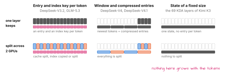
In Figure 17, the filled boxes are what a layer keeps for the request, and their number drops from left to right.

8.1 An Entry and an Index Key per Token#

The left side of Figure 17 is the design that we have used throughout this article. DeepSeek-V3.2 introduced this combination of MLA and sparse attention, and GLM-5.3 follows it, so everything from sections 2 to 4 carries over, including the choice between a copied and a split index. Only the concrete numbers differ. I haven’t looked those up for DeepSeek-V3.2, and I only tested my pull request with GLM-5.3.

8.2 A Window and Compressed Entries#

DeepSeek-V4, in the middle of Figure 17, goes one step further than sparse attention and doesn’t keep a full cache entry per token at all. Every layer keeps a sliding window with the last 128 tokens, plus a compressed version of everything older. Depending on the layer, this compressed cache has one entry for every 4 tokens, from which the indexer selects, or one for every 128 tokens, all of which attention reads.

For prefill, this design makes context parallelism particularly useful, and the SGLang post about DeepSeek-V4 explains why:

Most of DSv4’s hybrid attention path – SWA, C4/C128 compressors, indexer – can’t be sharded along heads, so TP hits a ceiling on long prompts.

(TP is tensor parallelism, SWA is the sliding window, and C4 and C128 are the two kinds of compressed entries.) So, this is the indexer problem from section 1.3 again, just with more modules that are not divided by head.

For decoding, I would expect a smaller gain, since much less grows with the number of tokens here than in an MLA cache, but I don’t have numbers for this. An open pull request for AMD GPUs nevertheless splits all of the state (the sliding window, both compressed caches, and the index), as on the right side of Figure 11. Each GPU therefore scores only its own compressed entries.

The part I like most is how that pull request deals with the additional collective that a split index needs. It all-gathers the queries (step 1 in Figure 9), so it packs each GPU’s best candidates into the same collective. This merges the collective that we estimated in section 4.3 with one that was already there.

DeepSeek-V4.1 compresses at lower ratios and, according to the SGLang post about it, produces the compressed entries and the index keys in only 4 layers that later layers reuse. Its prefill goes through the same context-parallel path as DeepSeek-V4. I found no pull request for decode context parallelism, and my guess is that a split index would be cheaper here, since only the few layers that select anything would need the additional collective.

8.3 A State of a Fixed Size#

In Kimi K3, on the right side of Figure 17, most layers keep nothing per token at all: only 24 of the 93 layers use MLA. The other 69 use a form of linear attention called Kimi Delta Attention (KDA), which keeps one state of a fixed size per request instead of a cache entry per token. It updates this state by going through the tokens in order.

For decoding, the KDA layers therefore have nothing to split, and decode context parallelism only applies to the 24 MLA layers, where it works as described in section 3. According to the SGLang post about Kimi K3, splitting the cache across 8 GPUs raised the number of tokens that they can hold from 1.5 million to 12.2 million. That’s about the factor of 8 that we would expect without an index.

For prefill, neither zigzag nor interleave works for a KDA layer, because it needs its tokens in order and the state that the earlier tokens left behind, so Kimi K3 currently uses pipeline parallelism for long prompts. A third layout, added by an open pull request and tested on a smaller model with the same kind of layers, goes back to consecutive pieces, as shown in Figure 18 below.

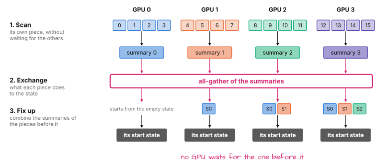
In Figure 18, each GPU first scans its own piece of the prompt without waiting for the others. The GPUs then exchange summaries of what each piece does to the state, and each GPU works out the state it should have started from. Such pieces are balanced for the KDA layers, since their cost is the same for every token. For the 24 MLA layers, though, they are as unbalanced as in section 2.2.

8.4 Where Things Stand#

Much of this is not merged. At the time of writing (October 2026), prefill context parallelism is merged for regular attention, DeepSeek-V3.2, the GLM-5 series, DeepSeek-V4, and DeepSeek-V4.1. Decode context parallelism is merged for MLA with regular attention, which includes Kimi K3’s MLA layers, and, on Ascend NPUs, for the sparse-attention models.

Everything else that I linked is still an open pull request: decode context parallelism for the sparse-attention models on GPUs and for DeepSeek-V4, the consecutive layout for KDA layers, and the draft that combines both features across two servers. So is a hand-off from a DeepSeek-V4.1 prefill server with context parallelism to an ordinary decode server. SGLang tracks all of this in two roadmap issues, one for prefill context parallelism and one for decode context parallelism.

On the question from section 4, the implementations for the sparse-attention models are divided. My pull request for Blackwell GPUs copies the index, and so do the one for Hopper GPUs and the merged path for Ascend NPUs, whereas a draft for AMD GPUs and the draft from section 5 split it.

9. What I Left Out#

To keep this article at a manageable length, I skipped a few things:

• Speculative decoding together with decode context parallelism, where the draft model keeps its own, unsplit cache.
• Storing the split cache in host memory or on disk when it doesn’t fit on the GPUs.
• Context parallelism across several machines. (For the sparse-attention models, SGLang limits it to one machine with at most 8 GPUs.)
• Pipeline parallelism, which only came up as the alternative in sections 5 and 8.

10. Summary#

To wrap up, let’s collect the answers to the three questions from section 1.5 in one place. Figure 19 below shows them for GLM-5.3 on 8 GPUs.

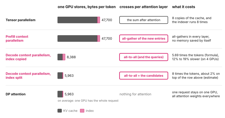
The thing to notice in Figure 19 is the first column. Prefill context parallelism leaves the bar untouched, and decode context parallelism shrinks it to 8,388 bytes per token with a copied index and to 5,963 bytes with a split one. DP attention averages the same 5,963, with a whole request on one GPU and nothing on the others, plus all the attention weights on every GPU.

So, coming back to the question from the beginning: one idea needs two implementations because the two phases have different bottlenecks. Prefill has too many queries, so it splits the queries and leaves the cache whole. Decoding has a single query and too many cache entries, so it splits the cache and leaves the work per step about the same.

The index is the part that I expect to matter more over time. With 2 or 4 GPUs, copying it costs little, but in rack systems such as the GB300, a single NVLink domain already spans up to 72 GPUs. If a tensor-parallel group were that wide and split its cache across all 72 with a copied index, the formula from section 4.2 would give 14.0 times the capacity instead of 72 times. The reason is that 82% of what each GPU stores per token would then be the index.

Contexts keep growing as well. A request with 1 million tokens would need about 42 GB of cache, and its prefill would have to go through 500 billion pairs, 61 times as many as for our 128,000-token prompt. Such a request needs both features at once, and that is the combination SGLang still rejects (section 5).