The Disaggregation Trap: Why Splitting Inference Across Specialized Chips Will Fail

TL;DR#

Over the past year, the AI infrastructure industry seems to have converted to a new paradigm: LLM inference is not one uniform workload, so we should saw the GPU in half and build a specialized computer for each phase.

Look at any roadmap this year and you see the same picture, with boxes and arrows drawn all over the data center:

• AWS pairs Trainium 3 for prefill with Cerebras CS-3 wafer-scale systems for decode, and sells it as a premium tier on Bedrock.
• AMD pairs its Helios (MI455X) racks with the Cerebras WSE-3 on the same split. It has also agreed to acquire Taalas (announced in August 2026), which hardwires a model’s weights directly into silicon.
• Startups such as d-Matrix (Corsair, digital in-memory compute) pitch dedicated cards for drafting, decoding or prefill.
• NVIDIA announced the GDDR7-based Rubin CPX for prefill in September 2025, then dropped it from the roadmap at GTC 2026. Its slot went to Groq 3 LPX racks, built on Groq technology licensed in a deal reported at about $20B. LPX runs the latency-critical part of decode, the FFN and MoE experts, while the Rubin GPUs keep attention. That is Attention-FFN Disaggregation (AFD).

On a marketing slide, the logic is very convincing. Prefill is compute bound and decode is memory-bandwidth bound. Why pay for expensive HBM bandwidth during prefill? Why let the Tensor Cores sit below 5% utilization during decode? Put each phase on its own specialized silicon, connect them with an RDMA fabric, and declare victory… Of course, the slide never shows the bill for that fabric.

Let me state my position up front. Once you put three things together, heterogeneous hardware disaggregation becomes an operational and economic trap:

1. the queuing math,
2. the workload dynamics of speculative decoding and multi-turn agents, and
3. the physical cost of moving data.

The substantive problem is that the pitch confuses a software scheduling optimization on fungible GPUs with a physical procurement commitment on non-fungible ASICs. Split Prefill, Decode, Draft and Verify (or some combination of them) onto dedicated heterogeneous chips, and five resource ratios get locked the moment you sign the purchase order. Yet the workload mix those ratios must serve keeps drifting along exactly those five dimensions: within a request, across the day, and across model generations over the four-to-five-year life of the hardware. Worse, you give up on-die locality and pay a heavy tax in network traffic, synchronization and duplicated HBM.

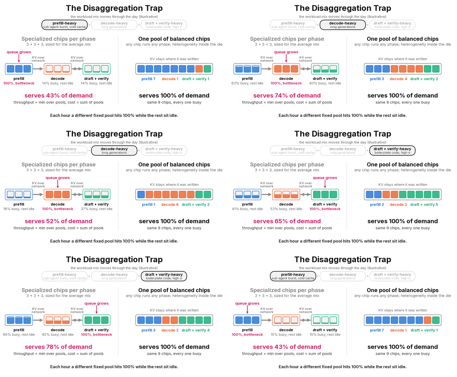
To be fair, specialization is not free money for the other side either. The real question is a break-even: does the specialized chip’s efficiency gain survive its lower average utilization and the boundary tax? I will write that inequality down in Section 3.4. My claim is that, for most fleets, it does not.

I believe OpenAI’s Jalapeño inference ASIC, presented at Hot Chips 2026, is the best example of the alternative. It puts the heterogeneous capability inside one balanced chip, instead of spreading it across a network that has to drag the KV cache around. The price is some dark silicon. OpenAI itself has not argued against disaggregation; this is my reading of the design. But idle die area costs far less than a stranded rack of the wrong chip, plus the network needed to feed it.

1. How a Scheduling Trick Became a Silicon Delusion#

To understand how the industry walked into this trap, we first have to separate two things that keep getting mixed up:

• software disaggregation on homogeneous hardware, and
• hardware specialization across heterogeneous pools.

Let’s start from the beginning. Early LLM serving systems used continuous batching, with prefill and decode sharing the same GPU. But the two phases look completely different:

• Prefill ingests thousands of prompt tokens in one large parallel GEMM.
• Decode advances each sequence by one token per step. Its GEMMs are skinny (M equals the batch size) and bound by memory bandwidth.

So when a long prefill arrives mid-flight, every in-flight decode sequence stalls for hundreds of milliseconds to seconds, and the p95 inter-token latency (ITL/TPOT) blows up. This is the classic prefill-decode interference problem.

If you were around when chunked prefill was introduced, you remember the fix. It slices long prompts into fixed token budgets and piggybacks decode tokens onto the same iteration, and every major engine ships it today. Of course, chunked prefill does not remove interference completely, because each chunk still adds to the decode step time. But it bounds that interference, and it does so without a network hop. A common rule of thumb is that below roughly 1,000 GPUs, chunked prefill on a shared pool is enough.

At hyperscale, and with large Mixture-of-Experts (MoE) models, software Prefill-Decode (PD) disaggregation took the next logical step (DistServe, Mooncake): prefill and decode run on separate pools of general-purpose GPUs, so each phase can use its own parallelism. DeepSeek’s current DeepInfer stack (October 2026) is the clearest example:

• Prefill runs on ordinary 8-GPU machines at the smallest expert parallelism that HBM allows (EP2–8 / DP2–8), using DeepEP’s high-throughput normal mode.
• Decode runs on 64–128-GPU supernodes at the largest expert parallelism available (EP64–128 wide-EP), using DeepEP’s low-latency mode and CUDA Graphs.

Note that even here the node shapes differ. But both sides are general-purpose GPUs running the same software stack, so a node can change roles without much work.

Homogeneous PD disaggregation works in production at DeepSeek, Moonshot (Mooncake) and other very large inference providers. So why does it work, economically and not just technically? Because the hardware is fungible. When daytime chatbot traffic gives way to nighttime RL rollouts or long-context agentic prefill, the scheduler drains a decode node and reprovisions it as a prefill node, or as a training node.

It is very tempting to assume that since the software roles were separated, the silicon should be specialized too. In practice, on real chips, that has meant:

• stripping memory bandwidth from prefill chips (Rubin CPX’s GDDR7), and
• stripping HBM capacity from decode chips (Groq LPX, Cerebras WSE, d-Matrix Corsair).

Problems start once the compute pools are no longer fungible, and that is exactly where specialization breaks down. In fact, the market is already dropping hints. Supply-chain reports from Ming-Chi Kuo in September 2026 say Rubin CPX is coming back for 2027 production, redesigned around 168 GB of HBM4 instead of GDDR7. Put bluntly, the bandwidth-stripped prefill chip did not survive contact with real workloads…

Conclusion: PD disaggregation works as a software decision precisely because the hardware underneath is interchangeable. Turning it into a silicon decision removes the very property that made it work.

2. Why the Two-Pool Mental Model Is Already Obsolete#

The whole case for splitting inference into a “compute chip” and a “bandwidth chip” rests on a simplified view of LLM serving with only two phases: prefill and decode.

But a request in a modern frontier inference stack does a lot more than prefill and decode. Production engines aim for interactive SLAs of 100–400+ tokens/s per user on 1T+ parameter MoE models, and to get there they rely on two things:

• speculative decoding (EAGLE-3, MTP, DFlash, DSpark), and
• agentic serving with high prefix-cache hit rates, e.g. long-running agents with interactive tool calls.

A single request actually passes through four distinct computational phases, and each one sits on a different limiting axis of the hardware roofline. Let’s go through them one by one.

1. Prefill: processes an input context of length T with hidden dimension d in one pass.

• The projections and the FFN scale as O(T·d²), and the full attention scores scale as O(T²·d).
• A large T gives the matrix engine a wide M dimension to amortize the weight loads, so prefill is matrix-compute bound. At very long contexts (100K+ tokens) it becomes KV-capacity bound as well.
• Its collective messages scale as O(T·d), so the communication is bandwidth bound rather than latency bound, which makes it easy to schedule smoothly.

2. Autoregressive Decode: each sequence advances one token per step.

• The matrix multiplies have M equal to the batch size, which is small, and they degenerate into GEMVs at batch 1.
• At short and medium contexts decode is weight-HBM-bandwidth bound. As the context grows, KV-cache reads overtake weight reads and it becomes KV-HBM-bandwidth bound. Where that crossover falls depends on batch size and attention type (GQA vs MLA).
• On top of that, every layer runs collectives with tiny messages, O(B·d) per step, which makes decode acutely bound by network synchronization latency.

3. Speculative Draft: what limits drafting depends on the draft architecture.

• Autoregressive drafters, i.e. classic draft models and EAGLE-3, run K serial steps at decode-like batch shapes. They are bound by draft-weight bandwidth and serial synchronization latency. For small draft heads, the target model’s large-vocabulary projection often dominates.
• Block-parallel drafters, such as the block-diffusion drafters DFlash and DSpark, propose all K positions in one pass. That moves the bottleneck to injecting the target model’s hidden states, the vocabulary projection, and sampling latency.

4. Speculative Verify: evaluates K+1 candidate tokens per sequence, or a dynamic token tree, in a single forward pass of the target model.

• For a dense model, verification reuses the weights across up to K+1 rows per sequence, which raises arithmetic intensity by up to a factor of K+1. In effect, it multiplies the batch size.
• For a sparse MoE model, that reuse collapses. The candidate tokens route to different experts, so the number of distinct active experts grows quickly with the verification budget. Verify then becomes bound by the bandwidth of those deduplicated expert weights and by bursty EP all-to-all traffic on the network.

Summarized into a table across the five hardware resource dimensions:

Inference phase	Matrix compute (FLOPs)	Weight memory BW	KV cache capacity & BW	Scale-up sync latency	Scale-out / EP all-to-all BW
Prefill	Extreme (bottleneck)	Low	High (capacity write)	Insensitive	Bandwidth-bound (smooth)
Pure decode	Minimal (under 5% utilization)	Extreme (bottleneck)	Extreme at long context	Extreme (per layer)	Latency/jitter-bound
Draft (EAGLE / block drafters)	Low	High (small footprint)	Low (local/windowed)	Extreme (K serial steps)	Minimal
Verify (MoE target)	Moderate–high	Extreme (deduplicated experts)	High (prefix reuse)	High	Extreme burst (incast)

As you can see, these four phases want incompatible ratios of compute, memory capacity, memory bandwidth and network latency. A dedicated chip per phase is not a family of big and small versions of one design. It is four different machines.

3. Why Fixed Hardware Ratios Always Lose#

Now suppose you buy the heterogeneous pitch and deploy a dedicated hardware pool for each phase. Once the racks are installed and cabled, the number of devices in each pool is fixed.

Let C = (C_P, C_D, C_S, C_V) be the service capacity of the Prefill, Decode, Draft (speculate) and Verify pools, and let W = (W_P, W_D, W_S, W_V) be the instantaneous demand each pool sees per committed output token. The throughput the whole data center can actually serve is then set by the most starved pool:

$$R_{\text{serviceable}} = \min_{i \in \{P,D,S,V\}} \frac{C_i}{W_i}$$

The problem is that W is not a stable property of your request mix. It swings at runtime, even within a single request.

3.1 The Speculative Acceptance Seesaw#

An output token can be committed in only two ways: pure decode, or draft + verify. Let φ ∈ [0, 1] be the fraction of output tokens committed through the speculative path, and R_out the total committed output tokens per second.

Each speculative round drafts K tokens, verifies them in one target pass, and commits E[n] tokens on average. Per unit of output, the pool loads are then roughly:

$$W_D \propto (1-\varphi)\,R_{\text{out}}, \qquad W_S \propto \frac{c_{\text{draft}}(K)}{E[n]}\,\varphi\,R_{\text{out}}, \qquad W_V \propto \frac{B_{\text{verify}}}{E[n]}\,\varphi\,R_{\text{out}}$$

Both φ and the verification load are driven by the token acceptance rate α. Assuming i.i.d. acceptance, the expected number of tokens committed per round is:

$$E[n] = \frac{1-\alpha^{K+1}}{1-\alpha}$$

And this expected value moves a lot with the workload:

• Structured code and boilerplate. α climbs to 0.85–0.95, so each verify pass commits several tokens. At α = 0.9 and K = 5, E[n] ≈ 4.7.
• Hard reasoning, rare entities, high-temperature sampling. α collapses, and most of each verify pass is thrown away.
• High concurrency. Speculation lives on spare FLOPs, and that slack disappears at large batch sizes. Drafting stays cheap, but the target model’s verification pass grows with the batch and quickly dominates the step.
• Adaptive schedulers. Under high load or low confidence they shorten the draft length or turn speculation off, which drives φ toward 0.

Now, where does this load actually land? There are two cases, and they should not be confused.

• The drafter is a head on the target model (MTP, EAGLE). This is how most production stacks run today. Draft and verify then sit on the same chip, and the seesaw lands inside the decode pool. At φ → 0 the hardware serves skinny, GEMV-shaped pure decode. At φ → 1 the same hardware must serve wide verify passes that touch many more distinct experts per step.
  • A general-purpose GPU absorbs both shapes.
  • A decode chip sized for one of them does not. Think of an SRAM part whose capacity was budgeted for batch-1 weights, which now sees verify’s deduplicated expert traffic.
• The drafter runs on separate silicon, for example a d-Matrix Corsair drafting next to GPUs. Then you get the full two-pool seesaw. The same users, model and context length can swing the load from the decode pool (φ → 0) to the draft and verify pools (φ → 1), with nothing more than a shift in α or in concurrency.

In the second case, you must size the decode pool for the φ = 0 peak, and the draft and verify pools for the φ = 1 peak. Those two peaks never arrive together. You pay CapEx and rack power for the sum of the peaks, but at any instant you only use one of the groups… In the first case the stranding is subtler: it shows up as a decode chip running far below its datasheet whenever the mix leaves the shape it was built for.

3.2 The Agentic Prefix-Cache Inversion#

The same whipsaw happens between prefill and decode.

In raw token terms, agentic coding traces are overwhelmingly input. Codex/SWE-bench Pro agent traces average a 131:1 input-to-output ratio; a typical session has 130,000 prompt tokens and 900 generated tokens, i.e. 144:1.

However, in any efficient serving system, prefix caching changes the picture completely:

• Prefill shrinks by an order of magnitude. Distributed prefix caches reach 92–95%+ hit rates on these traces. At a 92% hit rate only about 10,400 of those 130,000 prompt tokens are actually computed, and the effective ratio drops from 144:1 to about 11.6:1.
• Decode becomes capacity bound. The decode pool has to keep each request’s full ~131K-token KV cache resident in HBM for all 900 decode steps.

Then a wave of sub-agents spawns with fresh, uncached contexts, or the repository index changes, and the hit rate falls. A drop from 94% to 40% raises the uncached prefill work 10×, within seconds. This happens more often than you would think: harness bugs that break the cache, harness designs that do it on purpose, or simply a way of working that spawns fresh agents instead of forking ones that share a KV prefix.

3.3 Non-Fungible Silicon Locks Five Ratios#

In a homogeneous GPU cluster, when α shifts or the prefix-cache hit rate swings, the scheduler just moves workers between prefill, decode and verification. It is a configuration change, nothing more. (I am simplifying: rebalancing nodes on the fly is hard engineering. But it is software.)

In a physically disaggregated fleet, the idle chips are useless outside their own pool, even if your operations team wanted to move them:

• A GDDR7 prefill chip like the original Rubin CPX (about 2 TB/s of memory bandwidth, no NVLink) was never provisioned with the HBM bandwidth or the scale-up fabric that decode needs.
• An SRAM-only LPU with 500 MB of on-chip memory cannot hold a 128K-context KV cache, so it cannot help with prefill or attention either.

This leads to a consequence that is easy to miss: fixing the ratio of specialized device counts locks five resource ratios at the same time. Whenever one pool becomes the bottleneck, the others sit stranded, still paying for:

• depreciation,
• HBM and SRAM leakage power,
• optical transceivers and switch ports, and
• cooling.

3.4 But Doesn’t Scale Average It All Out?#

This is the strongest objection, so let’s take it seriously. α swings per request, but a big fleet serves millions of sessions at once. By the law of large numbers, per-request noise averages out, and the fleet-level ratio of prefill to decode to verify should be fairly stable. Then you could simply size each pool for the mean plus a buffer.

There are two problems with this.

First, the swings that matter are correlated, and correlated drift does not average out.

• Concurrency is a fleet-wide variable. When load rises, every adaptive scheduler trims speculation at the same time, so φ falls across the whole fleet together. That is exactly the moment the decode pool needs the most capacity.
• The mix moves as a whole. Daytime chat gives way to nighttime batch and RL rollouts. Sub-agent bursts arrive in waves.
• Model releases move it hardest. Served prompt lengths jump sharply in the weeks after a release, especially for an agent-oriented model, as users move from chatting with it to building agents on it. Together AI reports a jump of about 80% within two weeks.

Second, look at the timescale of the rebalancing.

• A homogeneous pool rebalances in minutes: drain a node and flip its role.
• A heterogeneous pool rebalances on the procurement timescale, which is quarters.

So the variance that matters is not the second-by-second jitter. It is the drift of the workload mix over the four-to-five-year depreciation life of the hardware. That drift includes architecture changes: dense to MoE, GQA to MLA to DSA sparse attention, separate drafters to MTP heads, 128K to 1M context. Rubin CPX is the textbook example: it was sized for a workload that changed before the chip shipped.

The best version of the pitch is a hybrid: buy specialized chips for the floor of each phase’s demand, and absorb the swings with general-purpose GPUs, the way a power grid runs base-load plants alongside peakers. That is a reasonable design, but look at what it gives up. The specialized pool now earns its keep only on the floor of its phase’s demand, and you have to forecast that floor four to five years out, across model generations that do not exist yet.

So we can write the break-even down. Cost per useful token is proportional to device cost over (performance × utilization). Define:

• g: the specialized chip’s performance-per-dollar gain on its own phase, after the boundary tax of Section 4;
• u_s: its average utilization over the hardware’s life;
• u_h: the utilization of a homogeneous fleet doing the same job.

Specialization wins only if:

$$g \cdot u_s > u_h \quad\Longleftrightarrow\quad g > \frac{u_h}{u_s}$$

Now a very simple calculation. If the fungible fleet sustains 70% and the specialized pool averages 40% across the drift, then g has to exceed 1.75×, net of the network, the duplicated HBM and the format translation. Vendors quote 3–5× and more, but almost always at the extreme interactivity point, on one model, at full utilization, and before the boundary tax. Very few of them publish u_s across a realistic year of traffic…

Conclusion: The throughput of a disaggregated fleet is the min over its pools, but its cost is the sum. When W drifts and C is frozen at the purchase order, you are paying for capacity you cannot use. Specialization has to clear g > u_h/u_s after the boundary tax, and the burden of proof sits with the vendor.

4. The Boundary Tax: KV Movement, HBM Duplication and the AFD Illusion#

Hardware disaggregation treats the network between chips as an afterthought. But moving data across that boundary mid-flight imposes two major physical taxes: moving the KV cache, and holding it twice.

4.1 The KV Transfer and HBM Duplication Tax#

When a request finishes prefill in pool A, its KV cache has to reach pool B before decode can continue. Layer-wise streaming hides part of the latency, but every single byte still has to cross the fabric.

The bandwidth wall. Modern MLA models compress the KV cache a lot, but agentic contexts more than make up for it. Let’s take GLM-5.3 as an example. Each of its 78 layers stores a 512-wide latent plus a 64-wide RoPE key, about 45 KB per token in FP8 (before the small extra key of the sparse-attention indexer). A 131K-token agent session therefore carries about 5.9 GB of KV.

Each turn only adds a few thousand tokens. But when a turn lands on a node that doesn’t already hold the session, the whole cache has to move (or be recomputed). A simple calculation:

• one move: about 120 ms of pure transfer over a 400G link (50 GB/s);
• 100 moves per second: about 590 GB/s, more than the entire scale-out bandwidth of an 8-NIC node.

HBM bandwidth interference. Reading gigabytes of KV out of the prefill node’s HBM and writing it into the decode node’s HBM is not free. It steals HBM bandwidth and NIC/PCIe cycles from the kernels running on both ends, and it competes with collective traffic on the same fabric.

The duplication tax. Under RDMA completion semantics, the prefill worker cannot free a request’s KV blocks until the decode worker confirms that the whole transfer has landed. By Little’s Law, every in-flight transfer is therefore held in both the prefill HBM and the decode HBM, and that duplicated footprint grows with transfer latency and request rate.

Now, to be fair: both taxes hit homogeneous PD disaggregation too. The difference is that on fungible hardware the scheduler has three escape hatches:

• move the work instead of the bytes, by routing the turn to the node that already holds the prefix;
• flip a node’s role, so the cache stays where it is;
• fall back to colocated chunked prefill when the KV traffic stops paying for itself.

On non-fungible pools there is no fallback. Decode can only happen on the decode chip, so the bytes must move, every time.

Crossing a vendor boundary then adds a tax that homogeneous fleets never pay. When GPU prefill feeds Cerebras, Gaudi or d-Matrix decode, there is no shared KV cache ABI. Block layouts (NHD vs HND), RoPE conventions and quantization scales all differ, so the cache has to be transposed and format-translated on the fly. Libraries like NIXL can carry the bytes, but someone still has to agree on what the bytes mean.

4.2 Case Study: The Death and HBM4 Resurrection of Rubin CPX#

Now for the elephant in the room: the death and revival of Rubin CPX.

In September 2025, NVIDIA unveiled Rubin CPX, a monolithic die built on the premise that prefill only needs FLOPs:

• 30 PFLOPS of NVFP4 compute (about 20 PFLOPS dense, per SemiAnalysis);
• 128 GB of inexpensive GDDR7 at about 2 TB/s;
• no NVLink: its off-chip I/O was 16 lanes of PCIe Gen6 into ConnectX-9 NICs on the scale-out network;
• power estimated at about 800 W.

It came in two configurations:

• Inside the compute tray (VR NVL144 CPX): 8 CPX next to 4 Rubin packages in every tray. That fixed the ratio at 2 CPX per Rubin package and pushed rack power to about 370 kW, versus about 190 kW for VR NVL144.
• As a separate CPX rack alongside an NVL144 rack.

Six months later, at GTC 2026, Rubin CPX was gone from the roadmap, and its slot went to Groq 3 LPX. NVIDIA gave no public explanation; reporting pointed to memory and substrate orders that never materialized. We can roughly infer what changed:

• The workload changed. Contexts grew toward 1M tokens, and agentic traffic moved from cold prefill to turns over heavily cached prefixes. Both make KV capacity and bandwidth matter, and 2 TB/s of GDDR7 behind nothing but PCIe Gen6 I/O is a poor fit for that.
• The network didn’t add up. All of CPX’s KV traffic had to leave over the same scale-out fabric that wide MoE expert parallelism already uses.
• The TCO didn’t add up. DRAM and GDDR7 prices were rising, and power and rack space in North American data centers were capped. Spending ~800 W and a rack slot on a card that could never help with decode or EP made little sense.

Then came the twist in September 2026. Supply-chain checks by Ming-Chi Kuo, the analyst best known for his Apple supply-chain calls, say Rubin CPX is coming back, with production starting in Q1 2027, but in a very different form:

• it drops GDDR7 for 168 GB of HBM4;
• its power envelope rises to 2,300 W, the same as the full Rubin GPU;
• it moves into standalone MGX racks, pairing 1:1 with Rubin GPUs that decode over Ethernet RDMA.

Obviously, NVIDIA has not given up on disaggregating prefill, and we should not pretend otherwise. But the cheap prefill chip is gone. To survive real workloads it had to take back expensive HBM and a full-size power budget, and at that point it looks a lot like a regular Rubin GPU, which moves g toward 1… The premise that prefill only needs cheap FLOPs did not hold up.

4.3 Case Study: Vera Rubin + Groq 3 LPX and the DDR Wall#

After dropping Rubin CPX at GTC 2026, NVIDIA moved to the other side of the split. It now pairs Vera Rubin NVL72 with Groq 3 LPX racks:

• 256 LPUs per rack;
• 500 MB of SRAM per LPU, so 128 GB of SRAM per rack;
• about 40 PB/s of aggregate SRAM bandwidth per rack, roughly 150 TB/s per LPU.

128 GB of SRAM cannot hold a long-context KV cache, so NVIDIA uses Attention-FFN Disaggregation (AFD). The Rubin GPUs keep the KV cache in HBM4 and run prefill and decode attention. At every MoE layer they hand the intermediate activations to the LPX rack, which runs the FFN and MoE experts.

Let’s work through the numbers for that loop using GLM-5.3, the model AgentX benchmarks.

Expert weights. GLM-5.3 has 75 MoE layers (78 in total, the first 3 dense), each with 256 routed experts and 1 shared expert. Each expert has 3 × 6144 × 2048 ≈ 37.7M parameters, or about 38 MB in FP8. Across 75 layers, the experts alone need about 728 GB.

SRAM capacity. A full LPX rack has only 128 GB of SRAM.

• Racks per model copy: about 6 (1,536 LPUs) at FP8, or 3 at 4-bit.
• A 2.8T-parameter model like Kimi K3.1 Pro needs about 11 racks even at MXFP4.
• The alternative is to stream weights from the 256 GB of DRAM attached to the Fabric Expansion Logic (FEL) on each LPX compute tray.

Now let’s trace the latency of a single MoE layer on LPX.

On-SRAM compute. If the experts are already sitting in SRAM, the work is tiny. A token’s nine active experts (about 340 MB) would stream out of a single LPU’s SRAM in about 2.3 µs at 150 TB/s, and in practice they are spread across many LPUs. Call it roughly 2 µs of operator time.

The network hop. Rubin dispatches tokens into the LPU’s FIFO (about 3 µs), the LPU computes (about 2 µs), and the result is written back (about 3 µs). Add EP combine and queueing, and the round trip comes to roughly 15–20 µs under ideal, jitter-free conditions.

The FEL DRAM bottleneck. One rack’s 128 GB of SRAM cannot hold 728 GB of experts, so each LPU holds a subset of layers and prefetches the next layer’s experts from the FEL’s DDR5.

• One rough estimate is that each LPU gets only 200–400 Gbps (25–50 GB/s) of that DRAM bandwidth, and the high end already assumes MRDIMM-12800.
• At 50 GB/s, loading one 38 MB expert takes about 755 µs.

Quite ironic, isn’t it? NVIDIA paid a reported $20B for Groq’s deterministic SRAM architecture to get ~2 µs expert execution, and in this configuration that execution stalls behind a ~755 µs DDR5 weight stream.

OK, but what if you “just buy the six racks per copy; hyperscalers buy hundreds of racks anyway”? That is fair. At scale this is a purchase, not a wall. But it is not free:

• each model copy now pipelines across six racks, so inter-rack hops join the per-token round trips;
• those racks only pay off if every copy runs saturated, which brings us straight back to the utilization term u_s in Section 3.4…

And even with all the experts resident, the activations still have to ping-pong between two domains, 75 times per generated token, once per MoE layer:

• an asynchronous HBM GPU domain on one side, and
• a synchronous, statically scheduled LPU domain with no backpressure on the other.

5. Heterogeneity Belongs Inside the Chip: The Dark Silicon Imperative#

If disaggregating across specialized chips strands capacity and floods the network, how do we solve the real problem? After all, even the best GPU stacks reach only about 10–15% of their theoretical HBM-bound decode speed at small batch sizes.

5.1 Why GPUs Stall at Low Batch#

Let’s start with why GPUs stall at low batch, and do a very simple calculation first. An 8-GPU B200 node has 64 TB/s of HBM bandwidth. GLM-5.x at NVFP4 moves about 21 GB of active parameters per token, so in theory batch-1 decode should reach about 3,000 tokens/s per user from HBM alone, with no exotic SRAM wafer required.

The measured results are far below that. On SemiAnalysis’s InferenceX AgentX benchmark (real coding-agent sessions, p90 per-user speed), the best published GLM-5.3 result on 8×B200 was 329 tokens/s per user as of November 2026. Together AI reports 417 with its new compiler (self-reported).

So where does the gap come from? The culprit is not HBM bandwidth. It is the GPU’s latency-hiding microarchitecture and its software launch model:

• Warp-occupancy dependence. A GPU hides memory latency by switching among tens of thousands of concurrent SIMT threads (warps). At batch 1 there simply aren’t enough independent warps to hide a ~400-cycle memory fetch, so the pipeline stalls and both the FLOPs and the HBM bandwidth go unused.
• The UMA and L2 partition tax. Dual-die Blackwell and Rubin present one unified memory space, so every SM reaches every HBM channel through a large L2 cache split into two partitions plus a global crossbar. zartbot estimates this adds 200–400 cycles of cross-partition latency, and in his view it caps effective HBM utilization at 60–70%.
• Kernel launch and barrier overhead. Launching thousands of small kernels per token throws away the on-chip register and shared-memory state at every boundary. DMA descriptor setup and mbarrier synchronization cost on the order of 100 cycles. That is a 2% tax on a 5,000-cycle training tile, but a 20% tax on a 500-cycle decode tile.

The strongest evidence is that removing just the software part of that tax already pays off on today’s fungible GPUs. Several stacks now run the whole decode pass as one persistent kernel instead of launching kernel by kernel:

• TileRT turns the entire decode loop into one persistent megakernel. On AgentX it holds the top single-user spot for GLM-5.3: 469 tokens/s per user on 8× MI355X in FP8 with MTP, more than 100 tokens/s ahead of the best GB300 NVL72 entry.
• SGLang and vLLM now ship the same idea. SGLang’s opt-in low-latency mode runs DeepSeek-V4.1-Flash decode through NVIDIA megakernel and AMD monokernel plugins, for up to 44% faster single-user decode on GB300 and 75% on MI350X. AMD reports that its MonoKernel cuts a GLM-5.2 decode step on 8× MI350X from about 2,459 kernel launches to 210 and runs 2.31× faster at batch 1. On the vLLM side, Inferact and Google built Kimi K3 megakernels for TPU v7x that plug into vLLM as a model runner; at launch they reached 391 tokens/s for a single user, against 251 on GB300.

The trade-off is throughput. These are batch-1 operating points, and engines tuned this way can’t serve large batches yet; for now they win a narrow use case. Still, they show that the gap to the roofline is mostly execution overhead, and that it is closing on homogeneous hardware. Ordinary software refreshes move the numbers just as fast: on Kimi K3, GB300’s tokens-per-dollar lead over TPU v7 grew from about 1.1–1.3× at launch to 1.5–2.6× after four NVIDIA software refreshes, within weeks.

Notice what this does to the break-even in Section 3.4. Every gain in compiled software lands on the fungible side of the inequality. It raises the baseline the specialized chip must beat, and it shrinks g. That alone is a reason to keep the fleet homogeneous. Redesigning the silicon is the next step, not a precondition.

OK, but what if you could fix the silicon as well?

5.2 Dark Silicon Is Cheaper Than Idle Accelerators#

Instead of moving the KV cache across a network between a prefill chip, a draft chip and a verify/decode chip, keep the KV cache local to one balanced chip and move the heterogeneity inside the die:

$$\text{External disaggregation} = \text{fixed active silicon} + \text{KV cache moving across the network}$$ $$\text{Internal heterogeneity} = \text{stationary, local KV cache} + \text{dynamically active silicon (power gating)}$$

Why is internal heterogeneity with dark silicon better than external specialized pools? There are three reasons.

First, idle pools cost almost as much as busy ones. An idle accelerator in a specialized pool still costs nearly all of its packaging, HBM stacks, SerDes, optics, switch ports, rack space and baseline cooling.

Second, dark silicon is cheap relative to a stranded accelerator. It is not free. A near-reticle N3P die is expensive, and a chip balanced for every phase is second-best at each one. But in an HBM4 package, the memory stacks, the advanced packaging and the power delivery take a large share of the bill of materials. The marginal tensor area is a fraction of that.

• Jalapeño’s compute die is near reticle size on TSMC N3P, with 13.4 PFLOPS of MXFP4.
• Some estimates put its tensor units at about 180 mm², or 22% of the die (though this detail isn’t central to the argument).
• Power-gating part of that array during memory-bound phases costs little, and the same chip can still bring all of its compute to bear when a prefill or wide-verify batch arrives.

Third, there is no stranding. Every chip in the cluster is identical, so all HBM capacity, HBM bandwidth and scale-up network stay fungible across all four phases. Nothing is stranded across pools when α drops or prefix-cache hit rates shift, and draft and verify never cross a network. In the language of Section 3.4, u stays close to u_h by construction.

5.3 A Blueprint for a Unified Inference Chip#

So how do you make one balanced chip good at both batch-1 latency (decode and draft) and large-batch throughput (prefill and verify)?

Borrow the latency-elimination playbook that CPU architects refined over thirty years, and pair it with AI-driven compilers.

1. Drop UMA and the giant L2; expose NUMA. Remove the large unified L2 cache and the global crossbar, and slice the chip into 64 core slices, each wired to its own share of the HBM4 interface:

• about 240 GB/s per slice (estimated), or 15.4 TB/s across the package;
• a hardware-managed L1 per slice, shared by the tensor, vector and scalar units, so data no longer shuffles between register files, shared memory, tensor memory and L2.

2. Replace warp multiplexing with an out-of-order core. A GPU needs dozens of concurrent warps to hide latency. Instead, use a CPU-style front end with hardware dependency tracking and L1 prefetch to extract instruction-level parallelism from a single instruction stream. At batch 1 that mechanism still works, because it never depended on thread concurrency in the first place.

3. Right-size the matrix units for small shapes. Large systolic arrays waste most of their area on padding at small M. Blackwell’s single-CTA tcgen05 MMA, for example, requires M of at least 64. Instead, use many smaller 64×64 broadcast-and-adder-tree arrays, estimated at fifteen per slice, with a latency of 6–9 cycles. These scale down efficiently to M = 1.

4. Add a dedicated on-chip collective network. Exposed NUMA means cross-slice reductions happen at every layer. A dedicated collective network-on-chip wired straight into each slice’s L1 hides the all-reduce and all-gather latency inside the tile-level GEMMs.

5. Let coding agents absorb the spatial-compiler complexity. NVIDIA spent a decade building hardware schedulers and unified caches because spatial NUMA programming is too hard for humans to do by hand. With LLM coding agents acting as auto-schedulers and auto-tuners over explicit layouts and a cycle-accurate simulator, static placement and prefetch scheduling become a search problem a machine can grind through. OpenAI credits LLM agents with part of Jalapeño’s post-silicon optimization.

---

Author’s Note

There are two caveats.

First, 216 GiB per package still does not hold a frontier model plus its long-context caches. Even OpenAI deploys Jalapeño 128 chips to a rack, so weights and KV are sharded across packages over the scale-up fabric. “Local” here means inside one homogeneous scale-up domain, not inside one die. But that is still a very different thing from shipping KV between non-fungible pools over scale-out RDMA.

Second, Jalapeño is co-designed with one lab’s models, even though it can run others. That is its own kind of specialization. But the fungibility argument still holds within that fleet: across phases, and across that lab’s model generations.

---

6. Conclusion: Don’t Put a Network Inside Your Inner Loop#

Let me be clear: software disaggregation of prefill and decode on homogeneous, fungible clusters is a legitimate tool. It earns its place when you operate thousands of GPUs and want to run narrow-EP prefill (EP2–8) separately from wide-EP decode (EP64–128).

Hardware disaggregation across specialized, non-fungible chip pools, however, is a trap for most fleets.

Split prefill, decode, draft and verify onto different physical computers, and you are betting your data center’s unit economics against three hard constraints.

First, workload non-stationarity. Several things swing the bottleneck across five resource axes:

• speculative acceptance rates (α),
• dynamic verification budgets, and
• agentic prefix-cache hit rates.

The swings that matter are correlated across the fleet and drift across model generations, so scale does not average them away. With fixed pools of specialized silicon, a large fraction of your capital is always sitting idle.

Second, the physics of data movement. Two patterns burn power, bandwidth and tail-latency budget that the specialized silicon then has to win back:

• moving multi-gigabyte KV caches across scale-out networks with no option to move the work instead, and
• ping-ponging activations ~75 times per token across a GPU/LPU boundary while streaming weights from external DDR5.

Third, the end of the human-compiler bottleneck. General-purpose GPUs struggle at low-batch decode largely because of the cost of human-friendly SIMT and UMA abstractions and kernel-by-kernel execution. Compiled and agent-tuned stacks are already removing much of the software part of that cost on today’s GPUs, and every such gain raises the bar a specialized chip must clear. Remove the hardware part as well, and a single HBM4 chip can reach 1,000+ tokens/s per user (OpenAI reports 700–1,459 for Jalapeño) while keeping the KV cache inside its own homogeneous scale-up domain. All it needs is an out-of-order core, a shared L1, and power-gated dark silicon.

Of course, most of the industry is betting the other way, with real money, and I could be wrong about specific fleets. A single-model, fixed-SLA, premium “fast mode” tier with very stable traffic is the one place where specialization most plausibly clears the bar. So don’t settle this with slides. Settle it with the inequality: does g > u_h/u_s hold, after the boundary tax, across a realistic year of your traffic and the next two model generations? If so, feel free to buy the chip.

Otherwise, the conclusion is very simple: keep the cluster homogeneous, keep the KV cache local, and push the heterogeneity inside the die. In the agentic era’s token factory, some waste from dark silicon is fine, but a stranded rack of specialized chips is a write-off.