If you look up how to serve a large Mixture-of-Experts model like GLM-5.3 in the SGLang cookbook, you find two kinds of recipes for the same 8 GPUs. The low-latency recipe uses tensor parallelism (--tp 8), where the large weight matrices are cut into 8 slices and all 8 GPUs work on every request together. The high-throughput recipe adds the flag --attn-dp-size 8, which turns on DP attention.
DP stands for data parallelism, and the idea is that the attention module is no longer split at all, so each GPU runs the whole attention module, but only for its own share of the requests. The Mixture-of-Experts (MoE) module, in which a small router picks a few of many expert networks for each token and which holds most of the weights, is still computed by all the GPUs together.
Why should that give more throughput? The usual answer is memory. A server keeps the keys and values of every token of every running request in its KV cache, and for a model like GLM-5.3, tensor parallelism stores a full copy of that cache on every GPU. I tried both layouts on 4 GPUs. With tensor parallelism, the 4 GPUs together can keep 2.7 million tokens of context, and with DP attention, they can keep 9.0 million.
However, the same experiment also shows a cost. A single request that is alone on the server gets a new token every 6.6 ms with tensor parallelism, but only every 12.2 ms with DP attention. That is surprising at first, because attention is the part that got simpler, and inside it, no GPU has to wait for another one anymore. So, where does the time go? What else does a server pay when every GPU keeps its own requests but still shares the MoE module with all the others, and at which load is that worth it?
In this article, I want to follow a request through a server with DP attention and stop at every place where “each GPU has its own requests” meets “all GPUs compute this together.” There are four such places, and each of them costs something different.
Everything I describe about how the mechanisms work comes from reading the SGLang source code, and I link the relevant files as we go. The numbers are for GLM-5.3, a model with 78 layers, in a version whose expert weights are quantized to 4 bits (NVFP4). All measurements are my own, on 4 of the 8 B300 GPUs (NVIDIA’s Blackwell generation) of a machine that I share with other people, which is why I use 4 GPUs and not 8. They don’t use speculative decoding, although the cookbook recipes do.
(This is the third article in a series, after How GPUs Talk to Each Other During LLM Inference and How GPUs Share a Long Context During LLM Inference, but you don’t need to have read the other two.)
1. Why Split by Request#
Why can 4 GPUs with tensor parallelism keep no more context than fits into the cache of one of them? The answer is the reason DP attention exists.
1.1 One Latent for All Heads#
In an attention layer, every token produces a key and a value. Since a token never reads the tokens after it, its key and value no longer change once they are computed, so a server stores them in the KV cache, which holds one cache entry per token in every layer.
Tensor parallelism distributes the attention heads across the GPUs. If each head has its own keys and values, a GPU that holds a quarter of the heads only has to store a quarter of each cache entry, and nothing is wasted.
GLM-5.3 doesn’t work this way, though. Like the DeepSeek and Kimi models, it uses Multi-Head Latent Attention (MLA), which compresses the keys and values of a token into one small latent vector that all 64 heads read. Tensor parallelism can split the heads and the large projection matrices, but it can’t split this vector, so every GPU stores the whole entry. The SGLang documentation describes the consequence as follows:
For example, DeepSeek models use MLA and only have one KV head. If we use tensor parallelism on 8 GPUs, it will lead to: […] Duplicated KV cache across all GPUs
(The previous article goes through the cache entry in more detail.)
1.2 What One GPU Holds#
So, what does tensor parallelism split in the attention module? It only splits the weights, which are the small part of what a GPU holds. The projection matrices of one attention layer of GLM-5.3 have 165 million parameters, which adds up to 24 GB for all 78 layers, whereas the cache of a busy server is several times as large. (I am using KB, MB, and GB for powers of 1,024 throughout this article.)
To see what this means for one GPU, I started the same model twice on 4 B300 GPUs with 269 GB each, once with tensor parallelism and once with DP attention. Figure 1 below shows what each server reported at startup.
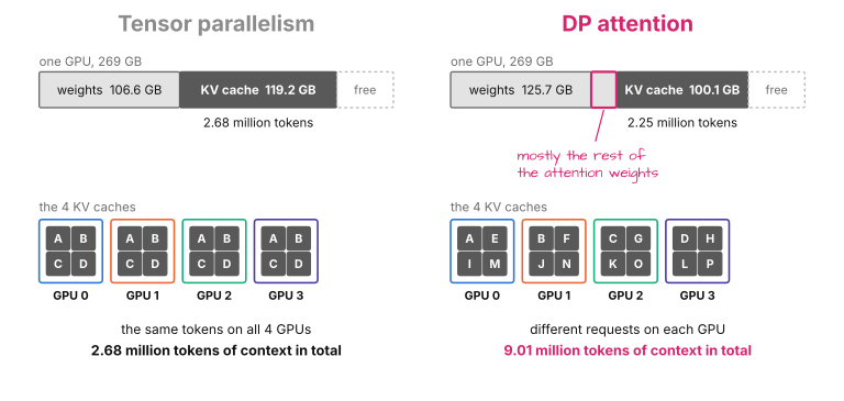
As we can see in Figure 1, a GPU holds 125.7 GB of weights with DP attention instead of 106.6 GB. Most of the difference is the three quarters of the split attention matrices that the GPU didn’t have before, since it now runs the complete attention module. This memory is taken away from the cache, which has room for 2.25 million tokens instead of 2.68 million.
The smaller cache is still the better deal, because with tensor parallelism, all 4 GPUs hold the same 2.68 million tokens. With DP attention, they hold 4 different sets of requests, which is 9.0 million tokens in total, or 3.4 times as many.
You may wonder why we don’t simply run 4 independent servers, one per GPU, if every GPU ends up with its own requests anyway. The reason is that the model doesn’t fit: the weights take 432 GB, most of it in the experts, and one B300 has 269 GB. So, the MoE module has to stay split across the GPUs, and that’s where the complications come from.
1.3 The Running Example#
To put numbers on these complications, I will count in rows. A row is the hidden state of one token position that the server processes in the current step (a step is one forward pass of the server), which for GLM-5.3 is 6,144 numbers of 16 bits each, or 12,288 bytes. A request that is decoding contributes one row per step, since it produces one token, and a prompt that is being read contributes one row per token.
With DP attention, each GPU has its own rows, so we can describe the server in one step by 4 numbers, the rows on each GPU. I will use five such situations:
- balanced: (16, 16, 16, 16), which is 64 requests decoding, 16 on each GPU
- single request: (1, 0, 0, 0)
- skewed: (40, 8, 8, 8), which is again 64 requests decoding
- short prompt: (512, 16, 16, 16), where GPU 0 reads a prompt of 512 tokens while the others decode
- long prompt: (4,096, 16, 16, 16)
The server has four places where the layout of attention (each GPU has its own rows) meets a layout in which all GPUs work on all rows. At each of them, I will ask the same three questions: what crosses between the GPUs, who has to wait for whom, and how many rows each GPU computes compared to the rows that are needed.
For tensor parallelism, the answers are short. What crosses is the sum of the partial results, twice per layer and for all rows. Everyone waits for everyone all the time, since all GPUs work on the same rows. And each GPU computes exactly the rows that are needed, so the ratio is 1.
Now, who decides which GPU gets which request?
2. One Scheduler per GPU#
In SGLang, the requests are dealt out by a small process called the controller. When DP attention is on, SGLang starts one scheduler process per GPU, and each scheduler has its own queue, its own batch of running requests, and its own KV cache. The controller sits between the HTTP server and the schedulers and hands each incoming request to one of them. By default, it does this round robin, without looking at the request at all: the first request goes to GPU 0, the second one to GPU 1, and so on. Figure 2 below shows the result for eight requests.
[Figure 2 is not drawn yet]
Figure 2 shows the first of two consequences that are easy to miss.
First, a request never moves. Request E is assigned to GPU 0 when it arrives, its cache entries are written there, and no other GPU ever sees them. This also means that the context of a single request can never exceed the cache of one GPU, which is 2.25 million tokens in our example.
Second, each scheduler also keeps its own prefix cache, the index that lets a new request reuse the cache entries of an earlier request that started with the same tokens. If the second turn of a conversation is dealt to a different GPU than the first one, it finds nothing to reuse there. On a busy server with round robin and 4 GPUs, that’s what happens about three times out of four, unless the client pins the request to a GPU via the routed_dp_rank field.
How much this matters depends on the workload. In an earlier experiment of mine with DeepSeek-V4.1-Flash on 4 B300 GPUs, where I replayed multi-turn agent sessions against a server with DP attention, round robin left 84% of the prompt tokens cached. When the client sent each session to the same GPU every time, it was 93%, and the output throughput at 128 concurrent sessions went from about 1,750 to 2,240 tokens per second.
This step is what produces the rows per GPU from section 1.3. If 64 requests arrive one after another and all of them are still decoding, round robin gives us the balanced situation, (16, 16, 16, 16). But requests finish at different times. The skewed situation, (40, 8, 8, 8), is what an unlucky mix of long and short requests can look like after a while, and each new prompt puts the server into one of the last two situations for a moment.
So, DP attention is 4 servers that share one MoE module, the one at the bottom of Figure 2. What happens where the two meet?
3. Around the MoE: Gather and Return#
This is where we find the first two of the four places, and I will call them the gather and the return.
3.1 Why the Rows Have to Travel#
The MoE module is still tensor-parallel, which means that each GPU holds a quarter of every expert. The output for a row is only complete once all 4 quarters have worked on it and their partial results have been added up. After attention, however, a row exists on one GPU only. So, the rows have to get to all GPUs before the MoE module, and the results have to come back afterwards.
For this, we need two operations in which all the GPUs take part. Such operations are called collectives, and since every GPU in the group participates, a collective is only finished once the slowest GPU is done. You probably know the all-reduce from tensor parallelism, where every GPU contributes a tensor of the same shape and every GPU ends up with the sum. The two that we need here are its siblings:
- In an all-gather, every GPU hands out the piece it has, so that every GPU ends up with all the pieces, one after the other. Nothing is summed.
- In a reduce-scatter, every GPU starts with a full-sized tensor, the tensors are summed across the GPUs, and each GPU only gets its own part of the sum back.
3.2 One Layer#
Let’s follow one layer in the balanced situation, where each GPU has 16 rows. Figure 3 below shows this with 2 rows per GPU, so that the individual rows are still visible.
[Figure 3 is not drawn yet]
Going through Figure 3 from left to right, each GPU first runs attention with all 64 heads on its own rows, and nothing crosses between the GPUs. Then, still by itself, it adds the attention output to the residual stream and applies the normalization that precedes the MoE module.
Next comes the all-gather. Each GPU hands out its 16 normalized rows, so that afterwards every GPU holds all 64 of them. Each GPU then runs its quarter of the experts on all 64 rows, which gives 64 partial sums. The reduce-scatter adds up these partial sums across the GPUs and gives each GPU back the 16 finished rows that belong to it, and the GPU adds them to its residual stream.
Note that only the normalized input of the MoE module is gathered, whereas the residual stream, shown as the gray line in Figure 3, never leaves its GPU.
In the code, the two collectives sit inside the boundary objects that connect the modules of a layer. Each of them wraps one module: before it, the object adds the previous module’s output to the residual stream, applies the norm, and moves the rows between the two layouts if needed. Below is a simplified excerpt (the full version is here):
# Simplified from DeepseekV2DecoderLayer.forward()
h = self.attn_boundary.prepare(h, forward_batch)    # add + norm, on this GPU's rows
h = self.self_attn(h, forward_batch)                # attention, this GPU's rows only
h = self.attn_boundary.finish(h, forward_batch)
h = self.ffn_boundary.prepare(h, forward_batch)     # add + norm, then the all-gather
with self.ffn_boundary.exit(forward_batch) as ffn_exit:
    h = self.mlp(h, forward_batch)                  # all rows, a quarter of each expert
h = ffn_exit.finish(h)                              # the reduce-scatter
3.3 The Same Bytes as Before#
In the balanced situation, the all-gather assembles 64 rows of 12,288 bytes each on every GPU, which is 768 KB, and the reduce-scatter sums a tensor of the same size.
With tensor parallelism, a layer has two all-reduces, one after the attention module and one after the MoE module, and with 64 requests, each of them also carries 64 rows. In other words, DP attention replaces two collectives per layer with two other collectives of the same size, so on paper, it doesn’t communicate any more than tensor parallelism does.
There is one difference that we will test in section 7, though. On this machine, SGLang doesn’t run the all-reduce of tensor parallelism through NCCL, NVIDIA’s general-purpose communication library. Instead, it uses a kernel from the FlashInfer library that writes directly into the memory of the other GPUs and also does the residual add and the normalization in the same kernel. (This fused kernel is the subject of the first article in this series.) SGLang turns the fused kernel off when DP attention is on, and the all-gather and the reduce-scatter are regular NCCL calls.
3.4 Summary#
To summarize in terms of our three questions for the balanced situation, what crosses are the 64 normalized rows before the MoE module and the 64 partial sums after it. Every GPU waits at these two collectives for the slowest one. And each GPU computes 64 rows in the MoE module for the 64 that are needed, so the ratio is 1.
The balanced situation is the convenient one, though. An all-gather needs a piece of the same length from every GPU, and a GPU can only take part if it knows how many rows the others have. So, how does it find out?
4. Agreeing on a Step#
The 4 schedulers are separate processes, and each of them decides for itself what its GPU should do next, so they have to come to an agreement before every single step. This agreement is the third of the four places, and it happens before the GPUs compute anything.
4.1 Recorded Steps#
A decode step consists of a long sequence of small GPU kernels, and for a small batch, launching them one by one from Python takes up a noticeable part of the step. A CUDA graph avoids this: at startup, the server runs a step once for a fixed number of rows and records every kernel launch, and later, it replays the recording instead of launching the kernels one by one.
A recording only fits the number of rows it was made for. The server therefore records a whole list of sizes, which I will call buckets, and rounds a batch up to the next bucket. For example, my server records 52 buckets for decoding (1, 2, 4, 8, 12, 16, 24, 32, 40, and so on up to 512), and it also records 42 buckets for reading prompts, from 4 to 2,048 rows. A step that fits none of the buckets runs the ordinary way, kernel by kernel, which is slower. I will call that an unrecorded step.
With DP attention, the all-gather and the reduce-scatter are part of the recording. This means that all 4 GPUs have to replay the same bucket, since a recording fixes the shape of every tensor in it, including the piece that a GPU hands to the all-gather. The startup log even says so for the prompt recordings:
Prefill CUDA graph captured a DP gather/scatter; DP ranks will replay a shared MAX_LEN bucket.
(In SGLang’s terms, prefill is the reading of a prompt, and a DP rank is what I have been calling a GPU with its scheduler.)
4.2 Ten Numbers#
Each scheduler therefore needs the row counts of the others, and all of them have to agree on whether to replay a recording. SGLang handles both with one small exchange. In every iteration of its loop, after a scheduler has picked its next batch, it packs ten integers into a tensor (the full version is here):
# Simplified from scheduler_components/dp_attn.py
torch.tensor([
    self.num_tokens,                        # my rows in this step
    self.num_tokens_for_logprob,
    int(self.can_run_decode_cuda_graph),    # my vote for the decode recording
    int(self.is_extend_in_batch),           # do I have a prompt?
    # ... six more, among them the vote for the prompt recording
])
An all-gather then hands these ten numbers from every scheduler to all the others. Note that this one doesn’t run on the GPUs but on the CPU: by default, it goes through PyTorch’s Gloo backend, which uses ordinary sockets between the processes.
Each scheduler now holds the same 40 numbers. The row counts become the 4 numbers from section 1.3. The votes are combined with a logical AND, so a recording is only replayed if every scheduler is fine with it. And “do I have a prompt” is combined with a logical OR, so that everyone knows when a prompt is being read anywhere. Since all schedulers compute the same thing from the same numbers, they arrive at the same decision without a coordinator.
4.3 A GPU with Nothing to Do#
Now, let’s apply this to the single-request situation, (1, 0, 0, 0). GPUs 1 to 3 have no requests at all. Can they sit this step out?
Unfortunately, they have to take part, because GPU 0 is about to enter an all-gather in every layer, and an all-gather in which a participant is missing never finishes. As long as any GPU has rows, a scheduler without requests creates an idle batch and runs the step anyway. And since the step is a recording for a fixed bucket, the idle GPUs replay the same bucket-1 recording as GPU 0, just on a row of padding, as illustrated in Figure 4 below.
[Figure 4 is not drawn yet]
As we can see at the bottom of Figure 4, all 4 GPUs run a full decode step. Each of them pushes one row through attention, and after the all-gather, each of them pushes 4 rows through its quarter of the experts, 3 of which are padding.
By the way, this is not a quirk of SGLang. vLLM, another inference engine, supports the same layout, and its documentation asks for the same thing: “empty ‘dummy’ forward passes” on all the GPUs that have no requests while any other GPU has one.
4.4 Summary#
To summarize in terms of our three questions, what crosses before each step are 40 integers. Every scheduler waits for the slowest scheduler’s loop, since the exchange is only complete when all four have sent their numbers. And for the single request, each GPU computes 4 rows in the MoE module for the 1 that is needed, so the ratio is 4.
The single request is just the extreme case of GPUs that have different numbers of rows. What happens in general?
5. When the Rows Are Unequal#
What does a step look like when one GPU has 40 rows and the others have 8, or when one GPU reads a prompt while the others decode? Figure 5 below shows one step in each of our five situations, and we will go through the three new ones.
[Figure 5 is not drawn yet]
The thing to notice in Figure 5 is that every step ends for all four GPUs at the same time. Let’s see why.
5.1 Skewed Decoding#
In the skewed situation, (40, 8, 8, 8), all GPUs are decoding, so all schedulers vote for the decode recording, and the only question is which bucket to use. SGLang takes the largest row count of any GPU, 40 in this case, and every GPU replays the bucket for 40 rows. The three GPUs with 8 requests fill their other 32 rows with padding.
After the all-gather, every GPU therefore holds 4 × 40 = 160 rows, of which only 64 belong to a request. The padding rows are not skipped, either. They go through the router and the experts like real rows, and their results are thrown away afterwards. That’s a ratio of 2.5.
How much does this cost? I pinned 64 decoding requests to the 4 GPUs in different ways and measured the time between two tokens of a request. With (16, 16, 16, 16), it is 24.9 ms, and with (40, 8, 8, 8), it is 29.0 ms, so every request is 17% slower although the server has the same work to do. With all 64 requests on one GPU, it is 30.7 ms. (These are requests with 1,024 tokens of real text as context, and each number is the mean of three runs that differ by about 0.1 ms.)
5.2 A Short Prompt#
Next, the short prompt: GPU 0 has a new request with a prompt of 512 tokens, and the other GPUs are decoding 16 requests each. (If GPU 0 had decoding requests of its own, they would get no token in this step, since a scheduler with a prompt runs the prompt first.)
A server doesn’t feed a long prompt through the model in one piece but in chunks of a fixed maximum size. With DP attention, SGLang divides this chunk size by the number of GPUs, since every GPU can read a chunk of its own in the same step. On my server, the startup log shows the adjustment:
DP attention is enabled. chunked prefill size is adjusted from 16384 to 4096.
A prompt of 512 tokens is a single chunk, and it fits one of the recorded buckets for prompts. However, a recording is only useful if all GPUs replay the same one, and three of our four GPUs want to decode. In my setup, SGLang solves this by relabeling: a decoding GPU presents its batch as 16 very short prompts of one new token each, which is allowed because a prompt step with everything but the last token in the cache computes the same thing as a decode step. Now, all 4 GPUs can vote for the prompt recording, and every GPU replays the bucket for 512 rows.
The price is the padding again. Every GPU processes 512 rows, so after the all-gather, the MoE module on each GPU sees 2,048 rows, of which only 512 + 48 = 560 are needed. That’s a ratio of 3.7.
The relabeling is not always possible, though. SGLang refuses it when a decoding batch contains a request with a grammar or with log probabilities, and also with speculative decoding or with the expert-parallel backends of section 9, both of which the cookbook recipe uses. The step then runs unrecorded, like the long prompt below.
5.3 A Long Prompt#
Finally, the long prompt. GPU 0 reads a chunk of 4,096 tokens, which is more than the largest recorded bucket of 2,048. The vote fails, and all 4 GPUs run an unrecorded step.
Padding every GPU to the one with the most rows would be expensive here, since the all-gather would have to carry 4 × 4,096 = 16,384 rows, or 192 MB, to transport the 4,144 rows that exist. That’s why, in an unrecorded step with a prompt, SGLang switches to an exact buffer. Each GPU allocates a zero-filled buffer that is as long as all rows combined and writes its own rows at its own offset. Then, the buffers are summed via an all-reduce. Since adding zeros doesn’t change anything, the sum is effectively a concatenation:
GPU 0 writes:   [ a a a a a a a a 0 0 0 ]      4,096 rows, then zeros
GPU 1 writes:   [ 0 0 0 0 0 0 0 0 b 0 0 ]      16 rows at offset 4,096
GPU 2 writes:   [ 0 0 0 0 0 0 0 0 0 c 0 ]
GPU 3 writes:   [ 0 0 0 0 0 0 0 0 0 0 d ]
all-reduce:     [ a a a a a a a a b c d ]      4,144 rows on every GPU
The buffer has 4,144 rows, or 48.6 MB, and every GPU computes exactly the rows that are needed. On the way back, the reduce-scatter can’t be used, since it returns equally long pieces. So, the partial sums are added up with another all-reduce, and each GPU copies out its own rows.
The ratio is 1 here, but this is the situation in which our second question matters most. The three decoding GPUs have 16 rows each, and in every one of the 78 layers, they wait in a collective for the GPU that pushes 4,096 rows through attention. For the 48 requests on those GPUs, this step takes as long as a prompt chunk and not as long as a decode step.
5.4 Summary#
To summarize in terms of our three questions, what crosses in a step is sized by the GPU with the most rows: a padded all-gather when a recording fits, and an exact buffer in an unrecorded step with a prompt. The GPUs with few rows wait for the GPU with many, in every layer. And the ratio of rows computed to rows needed is 2.5 for skewed decoding, 3.7 for the short prompt, and 1 for the long prompt, where the cost is the waiting instead.
After the last layer, the rows meet one more module that is split across the GPUs, and this one is split in yet another way.
6. The LM Head#
The last module of the model, the LM head, turns the final hidden state of a row into one score (a logit) for every entry of the vocabulary. For GLM-5.3, it is a single matrix with 154,880 × 6,144 entries, or 1.8 GB. By default, SGLang splits this matrix across the GPUs by vocabulary, so each of our 4 GPUs holds the weights for 38,720 vocabulary entries and can compute a quarter of the logits of any row.
This is the last of the four places, and the situation resembles the one before the MoE module: a GPU has its own rows but only a part of the weights. It can either bring the rows to the weights or keep all the weights with the rows. Figure 6 below shows both, with two variants of the former.
[Figure 6 is not drawn yet]
6.1 Rows to the Weights#
The default, on the left side of Figure 6, repeats the pattern from section 3. First, the final rows of all GPUs are gathered with the exact buffer from section 5.3, so that every GPU holds all 64 of them in the balanced situation. Each GPU multiplies them by its quarter of the head. An all-gather then hands the quarters around, after which every GPU holds the complete logits of all 64 rows and copies out the 16 rows that are its own.
That’s 64 × 154,880 logits on every GPU in order to keep 16 × 154,880 of them. The ratio from our third question is therefore 4 here, even in the balanced situation.
The variant in the middle of Figure 6 avoids this waste with a collective that we haven’t used so far, the all-to-all, in which every GPU sends a different piece to each of the other GPUs. After the multiplication, GPU 0 holds a quarter of the logits for all 64 rows. Instead of handing all of it to everyone, it sends GPU 1 only the rows of GPU 1, GPU 2 only the rows of GPU 2, and so on, so that each GPU ends up with the full logits of its own rows and nothing else.
The pull request that added this variant measured the LM head of DeepSeek-V4 Pro on 8 B200 GPUs with 36 requests per GPU at 169 microseconds instead of 278.
The all-to-all needs the same number of rows on every GPU, though, and a step in which the row counts differ falls back to the all-gather. By default, SGLang only turns it on on servers that do nothing but decode, which we will meet in section 8.
6.2 Weights with the Rows#
The other choice, on the right side of Figure 6, is --enable-dp-lm-head. Every GPU then loads the whole head and computes the logits of its own rows by itself, so nothing crosses at all. On my server, this costs 1.3 GB of additional weights per GPU.
So, why isn’t this the default? According to the same pull request, the full head is slow when a GPU has few rows. With 36 rows per GPU, the multiplication by the whole matrix took 320 microseconds, which is more than the 278 of the split head including its all-gather. My guess is that this is because a GPU has to read all 1.8 GB of the matrix no matter how few rows it has, and I would expect it to turn around when a GPU has many rows. In practice, all DP attention recipes for the NVFP4 version of GLM-5.2 in the open InferenceX benchmark turn it on.
6.3 A Hang That Came with the All-to-All#
Recording a collective into a CUDA graph can also go wrong, and the all-to-all is an example.
NCCL can register the send and receive buffers of a recorded collective, so that the GPUs later move data through these registrations directly. The all-to-all of the LM head, however, runs on temporary buffers from the memory that belongs to the recording, and the same addresses are also handed to other tensors. A docstring in the SGLang source describes what happened then:
[…] the registered exchange does not survive that: under a burst of new requests (DP ranks ramping at different rates) one rank finishes its step while the others spin in ncclDevKernel_SendRecv forever, and every DP rank hangs.
The fix is the environment variable NCCL_GRAPH_REGISTER=0, which SGLang now sets by itself whenever the all-to-all is active. It’s the same problem that we keep running into: a collective only ends when every GPU has done its part.
6.4 Summary#
To summarize in terms of our three questions for the default, what crosses are the final rows and then the logits, a quarter at a time. Everyone waits at two more collectives per step. And each GPU ends up with 4 times the logits it needs. The all-to-all brings this ratio back to 1, and the full head removes the communication altogether.
These were the four places where the two layouts meet: the gather before the MoE module, the return after it, the agreement before each step, and the LM head. With that, we can come back to the question from the beginning.
7. Where One Request’s Time Goes#
In the introduction, a single request got a token every 6.6 ms with tensor parallelism and every 12.2 ms with DP attention. Which of the four places takes the 5.6 ms?
Before I measured anything, my guess was the collectives. A step has 78 layers with 2 collectives each, so the difference would be explained if each of the 156 calls into NCCL were about 36 microseconds slower than its share of the fused kernel. The other candidates were the exchange before each step, the LM head with its two additional collectives, and the 3 rows of padding in the MoE module.
To find out, I did two things. First, I recorded a trace of every GPU kernel during 40 decode steps of a single request, once for each layout. Second, I ran the same single request against servers that each differ from the default in one flag. Figure 7 below shows both results.
[Figure 7 is not drawn yet]
Let’s start with the top of Figure 7. One caveat first: kernels on a GPU overlap in time, so the bars are longer than a step and their segments are not exact shares of it. They add up to 10.5 ms for tensor parallelism and 16.5 ms for DP attention, a difference of 6.0 ms.
The collectives are the blue segments. With tensor parallelism, the fused kernel takes 1.1 ms per step, including the add and the normalization. With DP attention, the all-gather and the reduce-scatter take 1.7 ms together (about 11 microseconds per call), and the add and the normalization, which now run as a kernel of their own, take another 0.7 ms. That’s 1.3 ms more, about a fifth of the difference. So, my guess was mostly wrong.
More than half of the difference, 3.3 ms, is in the first segment, the matrix multiplications outside of the experts. A recorded step doesn’t tell us which line of Python a kernel belongs to, but there is only one group of large matrices that changed between the two layouts: the attention projections, of which the GPU now multiplies the whole matrix instead of a quarter. I assume that for a single row, such a multiplication is limited by reading the weights from memory, and with DP attention, the GPU that holds the request reads all 24 GB of attention weights in every step.
In other words, the single request is slower mainly because it has lost three of its four GPUs for the attention module. That’s the price that section 1 already announced, and it has little to do with the four places.
The second segment is the multiplications inside the experts, which go from 1.3 to 2.5 ms. This one does come from the gather: with tensor parallelism, each GPU pushes 1 row through its quarter of the experts, and with DP attention, it pushes 4, of which 3 are padding. So, the ratio of 4 from section 4 adds about 1.1 ms of kernel time here.
The bottom of Figure 7 looks at the same question from the other side. If I take the fused kernel away from tensor parallelism, a token takes 6.8 ms instead of 6.6, and only when its all-reduce goes through NCCL does it take 9.3 ms. (NCCL’s all-reduce is evidently much slower for these small messages than the all-gather and the reduce-scatter that DP attention uses.) On the DP attention side, none of the switches changes much. Putting the whole LM head on every GPU makes a token slightly slower, in line with section 6.2. Returning the rows with an all-reduce and a copy instead of the reduce-scatter saves 0.4 ms, and moving the exchange from the CPU to the GPUs costs 0.8 ms. (I didn’t measure the exchange by itself.)
There is a consolation in these numbers, though. If the three idle GPUs replay the step anyway, giving them requests costs almost nothing: with one request on each of the 4 GPUs, a token takes 12.5 ms instead of 12.3. (These two numbers are from the test in section 5.1.) A server with DP attention is slow for one request, but it is about as slow for four.
So, that’s a server with very little to do. The other costly situation was a prompt that arrives next to requests that are decoding.
8. A Prompt in the Way#
How much does a prompt on one GPU slow down the requests that are decoding on the other three, and what can be done about it?
8.1 What the Other GPUs Notice#
To measure this, I recreated the two prompt situations from section 5 on my server. I pinned 16 decoding requests to each of GPUs 1, 2, and 3, let them run alone for a while, and then sent a prompt to GPU 0 every half second. For every token of the decoding requests, I recorded the time since the previous token of the same request. Figure 8 below shows the result in its first row, together with a second test that we will get to in a moment.
[Figure 8 is not drawn yet]
Alone, a token arrives every 24.1 ms. With the short prompts, most tokens still do, but each prompt causes two slow steps of about 40 ms. That’s the padded recording from section 5.2, in which every GPU computes 512 rows, and overall, the three GPUs produce 6% fewer tokens.
With the long prompts, each prompt causes two slow steps of about 150 and 90 ms, where a decode step takes 24. Since this happens every half second, the 48 requests on the other GPUs produce 38% fewer tokens, although none of the prompts is on their GPU. This is the waiting from section 5.3, and the SGLang documentation has a name for it, DP attention imbalance.
Is tensor parallelism better off? There, a prompt is in the way of everyone by design, since the server has a single scheduler that runs either a prompt step or a decode step. For the second test, I therefore didn’t pin anything: 64 requests decode, and 4 prompts per second arrive wherever the server puts them. Rows 2 and 3 of Figure 8 show both layouts. With prompts of 4,096 tokens, the slowest steps take 162 ms with tensor parallelism and 180 ms with DP attention, and the decoding requests lose 54% and 50% of their tokens. So, in this test, DP attention doesn’t shield a GPU from the prompts of its neighbors, but tensor parallelism has the same problem to the same degree.
8.2 Three Ways to Change the Rows#
What can be done about this? All the remedies that I found in SGLang work the same way: they change the rows per GPU that a step has to deal with.
The first one we have already seen. Since the chunk size is divided by the number of GPUs, the largest entry that a prompt can put into a step is 4,096 rows here and not 16,384. This limits how long a single step can keep the other GPUs waiting, and it means that a long prompt takes more steps.
The second one is the prefill delayer, which is off by default and enabled with --enable-prefill-delayer. With it, the schedulers exchange a few more numbers before a prompt is started, and a GPU that has a prompt waits until every GPU has one, for at most 30 passes of the scheduler loop. The idea is illustrated in Figure 9 below.
[Figure 9 is not drawn yet]
On the left side of Figure 9, each of the four prompts causes a slow step of its own, during which the three other GPUs wait. On the right side, the four prompts are read in the same step, so the requests that are decoding are held up once instead of four times. In terms of our situations, four steps like (4,096, 16, 16, 16) become one step with (4,096, 4,096, 4,096, 4,096). The price is that the first prompt has to wait for the last one.
In the unpinned test from above with prompts of 4,096 tokens, the delayer made the slow steps rarer but longer (233 ms, the last row of Figure 8). The requests that were decoding produced 1,610 tokens per second during the prompts instead of 1,270, and a prompt took 0.65 seconds instead of 0.30.
The third remedy is to not mix the two kinds of work at all. In a disaggregated deployment, one server only reads prompts and hands the finished KV cache to a second server that only decodes. The decode server then never sees a prompt, and with a well-balanced load, it stays in the first of our five situations. The InferenceX recipes for GLM-5.2 are built this way, with DP attention on the prefill server, where every GPU is reading prompts anyway, and either DP attention or plain tensor parallelism on the decode servers, depending on the load.
All three remedies leave the gather in place and only change what goes through it. Can we get rid of the gather itself?
9. Expert Parallelism: No Gather Around the MoE#
The gather exists because every GPU holds a quarter of every expert, so every row has to visit every GPU. With expert parallelism (EP), each GPU holds a quarter of the experts, which is 64 of the 256 in our example, but holds them in full. A row then only has to visit the GPUs that hold the 8 experts that the router picked for it. Sending each row to those GPUs is called dispatch, and sending the results back to the GPU that the row came from is called combine. Both are all-to-all operations, and SGLang delegates them to a backend that is selected via --moe-a2a-backend. (The first article in this series has a section on these backends.)
For DP attention, this is a natural fit, since the rows have to travel anyway. Figure 10 below shows the MoE module of one layer in both layouts.
[Figure 10 is not drawn yet]
As we can see on the right side of Figure 10, there is no all-gather and no reduce-scatter anymore. When an all-to-all backend is set, the code that sits between attention and the MoE module simply does nothing across GPUs, and a row leaves its GPU inside dispatch and comes back inside combine.
What does this do to the ratio from our third question? A padding row is never dispatched to an expert, so the experts only compute rows that are needed, and for them, the ratio goes back to 1 in every situation. (The router and the one shared expert that every row passes through still run on a GPU’s padding rows.) The rest stays, though. With the cookbook recipe, the recorded step still pads the attention module of every GPU to the one with the most rows, the schedulers still exchange their ten numbers, an idle GPU still runs every step, and the LM head is unchanged.
There is one more detail. GLM-5.3 has 3 layers at the bottom whose feed-forward module is an ordinary dense one without experts. These keep the gather and the return unless we pass --moe-dense-tp-size 1, which gives every GPU a full copy of them. (And as mentioned in section 5.2, a short prompt next to decoding GPUs runs as an unrecorded step here.)
{{ep_measured_paragraph}}
So, we now have all the pieces. Let’s see how they add up across the whole range of loads.
10. When It Pays Off#
At which load does the trade turn around? To find out, I ran both layouts with real text, the first turns of ShareGPT conversations as prompts and 256 output tokens per request, at 1 to 256 concurrent requests. (These prompts are short, a few hundred tokens for most of them, so this is a chat-like load in which almost all of the time goes into decoding. Each point is the mean of three runs.) Figure 11 below shows the result.
[Figure 11 is not drawn yet]
Let’s read Figure 11 from left to right. For a single request, tensor parallelism produces 157 tokens per second and DP attention 81, which is the factor of 2 from section 7. Up to 64 concurrent requests, tensor parallelism stays ahead, by 15% at 64 (2,880 against 2,500 tokens per second). At 256 concurrent requests, the order has turned around: DP attention produces 6,400 tokens per second and tensor parallelism 4,680, which is 37% more. The time per token tells the same story, since at 256 requests a token takes 35 ms with DP attention and 49 ms with tensor parallelism. (The 99th percentile on the right is closer: 50 against 60 ms, with a spread of 38 to 60 ms between the three runs of DP attention.)
So, on this machine and with this load, the crossover is somewhere between 64 and 256 concurrent requests, or between 16 and 64 requests per GPU.
Why does DP attention win at the high end? It’s not the cache, since 256 requests of a few hundred tokens fit into either layout many times over. And on paper, the GPU work is the same, because a GPU with a quarter of the heads for 256 requests has as much attention to compute as a GPU with all the heads for 64. What does differ is the CPU side: with tensor parallelism, a single scheduler process prepares, samples, and bookkeeps a batch of 256 requests for every step, whereas with DP attention, four processes each handle 64. My guess is that this is where most of the 14 ms go, but I haven’t verified it.
The green line in Figure 11 is the middle setting, 2 attention groups of 2 GPUs each (section 11 shows how to ask for it). I expected it to land between the other two, but it is slightly behind DP attention at every point that I measured, with 12.6 ms per token for a single request. So, on 4 GPUs, it buys cache (twice that of tensor parallelism) but no speed.
There are two more things that the figure doesn’t show. The first one is the time to the first token. With requests arriving at random, 4 per second on average, the first token takes 47 ms with tensor parallelism and 86 ms with DP attention, presumably since the prompt of a request is also read by one GPU instead of four.
The second one is the cache, which was the reason for all of this in the first place. As soon as the requests are long, tensor parallelism runs out of room first. With 32,000 tokens of context per request, its 2.68 million tokens are enough for 83 requests, whereas the four caches of DP attention hold 70 requests each, 280 in total. I didn’t run this case here, but the previous article has a sweep at that length from the same kind of machine, in which tensor parallelism couldn’t hold 128 requests and DP attention was still gaining throughput at 256.
What about the two recipes from the introduction? They differ in more than the layout, since both use speculative decoding with different settings, and the low-latency one limits itself to 16 requests. Run as written in the cookbook for 4 GPUs, the low-latency recipe produces 318 tokens per second for a single request and the high-throughput recipe 152, and at 16 concurrent requests, it is still 1,620 against 1,280. The high-throughput recipe then keeps scaling up to 5,780 tokens per second at 256 concurrent requests, which is beyond what the other one accepts. {{cook_ht_tp_sentence}}
So, my rule of thumb after these measurements is the following. If a GPU will rarely have more than a few dozen requests and they fit into the cache, tensor parallelism is faster in every respect. DP attention is for the server that is full: many requests per GPU, or requests that are so long that the cache is what limits the batch. And a server with DP attention should not be judged by its single-request speed, since that’s the one thing it is bad at.
Please keep in mind what these numbers are, though: one model, 4 GPUs of one machine that other people were using at the same time, synthetic arrival patterns, and no speculative decoding except in the two recipes.
11. The Flags: --tp Is the Total#
How do we ask SGLang for these layouts? The flags are easy to misread, mostly because --tp is the total number of GPUs of the server and the other flags divide it.
--attn-dp-size divides the GPUs into attention groups. So far, each group was a single GPU, but a group can be wider. With --tp 8 --attn-dp-size 2, there are 2 groups of 4 GPUs each. Inside a group, attention is tensor-parallel again, so 4 GPUs work on a request and its cache entries are stored 4 times, and the requests are divided between the groups as in section 2. The MoE module divides the same 8 GPUs in its own way. Figure 12 below shows four deployments.
[Figure 12 is not drawn yet]
The first row of Figure 12 is the mixed case, which contains a detail that I find quite neat. Inside a group, attention needs an all-reduce to add up the partial results of its 4 GPUs, and SGLang folds this all-reduce into the gather. A reduce-scatter inside the group leaves each GPU with a quarter of the group’s finished rows, and a single all-gather over all 8 GPUs then assembles the buffer for the MoE module.
The second row is the high-throughput recipe for the FP8 version of GLM-5.3 from the cookbook, which combines DP attention with expert parallelism (shown here without the flags for speculative decoding and memory):
sglang serve \
  --model-path zai-org/GLM-5.3 \
  --tp 8 \
  --attn-dp-size 8 \
  --moe-a2a-backend deepep \
  --chunked-prefill-size 32768 \
  --max-running-requests 256
Note that there is no --ep-size in this command, since choosing an all-to-all backend makes the expert-parallel width equal to --tp. Also, the chunk size is the budget for all GPUs together, so each GPU reads 4,096 tokens per chunk here, and the limit of 256 requests means 32 per GPU.
The third row is a decode server from the InferenceX recipes for GLM-5.2 on 16 GPUs. It uses 16 groups of one GPU on 4 machines, expert parallelism over all 16, the full LM head, and --moe-dense-tp-size 1. Nothing in a layer is tensor-parallel anymore, and according to the source code, each GPU then picks the bucket for its own batch, so the padding to the GPU with the most rows is gone, while the exchange and the idle steps remain.
The fourth row is an example from the SGLang documentation for Kimi K3 on 32 GPUs. There, each of the 4 groups has 8 GPUs, and --dcp-size 8 additionally splits the cache of a group across its 8 GPUs. This is decode context parallelism, the topic of the previous article.
(If you come across --dp-size N --enable-dp-attention in older recipes, that’s the previous spelling of --attn-dp-size N. It still works but prints a deprecation warning.)
Two things happen without a flag. First, SGLang multiplies --schedule-conservativeness by 0.3 when DP attention is on, which makes each scheduler admit new requests more readily. Second, with --enable-metrics and the environment variable SGLANG_ENABLE_METRICS_DP_ATTENTION, the server exports statistics about the rows per GPU in each step and about the time spent waiting in the exchange.
Finally, a few architectures reject DP attention at startup (MiniCPM and ERNIE 4.5 VL, for example), and some forms of speculative decoding can’t be combined with it.
12. What I Left Out#
To keep this article at a manageable length, I skipped the following:
- Speculative decoding together with DP attention. The cookbook recipes use it, and some of the mechanisms above behave differently with it.
- Running several independent copies of a server behind a gateway, which is the natural choice when the model fits on one GPU.
- Disaggregated serving beyond the paragraph in section 8.
- What happens to the other GPUs when one of them fails.
- Whether the outputs are bit-identical to those of tensor parallelism, which I didn’t test.
- Two flags that are sometimes listed next to DP attention,
--enable-attn-tp-input-scatteredand--disable-attn-tp-gather. According to the source code, both of them concern tensor-parallel attention. --enable-dp-attention-local-control-broadcast, which changes how control messages reach the schedulers. (I did try it, and it made no measurable difference for a single request.)
13. Summary#
To wrap up, let’s collect the answers to the three questions in one place. Figure 13 below shows the five situations once more, this time with what I measured for each.
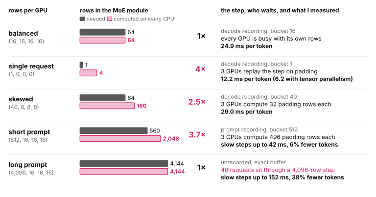
The thing to notice in Figure 13 is that the ratio in the middle and the measured cost on the right don’t go together. The single request has a ratio of 4 and pays about 1 ms for it, out of 5.6 ms that mostly come from having one GPU for attention instead of four. The long prompt has a ratio of 1 and is the most expensive situation for the requests that are decoding, since they wait.
So, coming back to the questions from the beginning: the time of the single request goes into the attention module itself, which a single GPU now computes alone, and only to a small part into the places where the two layouts meet. What a server pays there shows up under load. Every step is as long as the step of its busiest GPU, a skewed batch costs 17%, and a long prompt on one GPU takes more than a third of the tokens away from the requests on the other three. In return, the 4 GPUs keep 3.4 times as much context, and from somewhere between 16 and 64 requests per GPU, the server produces more tokens than with tensor parallelism.
What I find most interesting is how these costs change with the number of GPUs, since the cookbook recipe uses 8 and the InferenceX recipes 16. The arithmetic of this article carries over directly. With a tensor-parallel MoE module, a single request on 8 GPUs means 8 rows for 1 that is needed, and on 16 GPUs, it is 16. A step is as long as the busiest of 8 or 16 GPUs, and the more GPUs there are, the more likely it is that one of them has just received a prompt. I haven’t measured either of these, but it would explain why the recipes for 16 GPUs go to such lengths to remove the gather, replicate the dense layers and the LM head, and keep the prompts on a different server altogether.