What Matters in a ModelOpt Quantization Recipe

If you browse the popular open-weight models on Hugging Face these days, you will often find, next to the original, a second version whose name ends in -FP8 or -NVFP4. These are quantized checkpoints, which store the weights with fewer bits than the 16 of the original format, BF16. NVIDIA produces its own with a library called Model Optimizer (ModelOpt for short), and most of them go through one script, hf_ptq.py.

If we want such a checkpoint for a model that doesn’t have one, the script asks us for a recipe, and a recipe has four things to fill in. The first is the number format, separately for the weights and for the values that flow through the model at run time, the activations. The second is the scope, that is, which layers get the format. The third is the algorithm that picks the stored numbers. And the fourth is whether the KV cache, the memory in which the server keeps what it has computed for earlier tokens, is stored with fewer bits as well.

I filled in these fields in many ways for one model, Qwen3-8B, served most checkpoints with SGLang on a B300 GPU, and measured the size, the speed, and the accuracy. For accuracy, I used the perplexity on a standard text, where lower is better, and the share of problems solved on a math benchmark, GSM8K. Figure 1 below shows all of it at once.

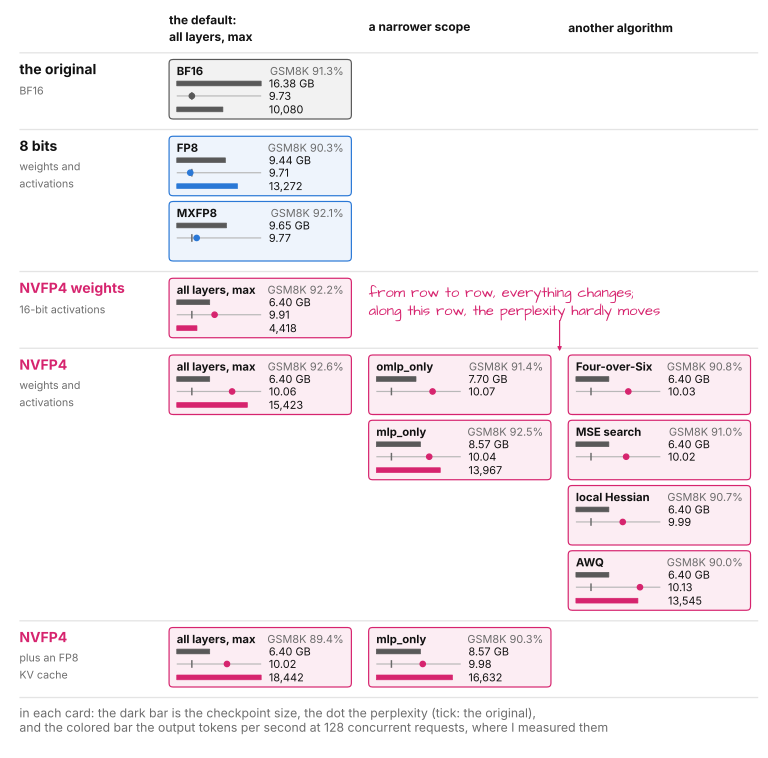
Figure 1 already shows the result. From row to row, the size, the speed, and the accuracy all change. Along a row, the perplexity hardly moves, and size and speed only get worse.

The rows are the format. FP8 made the model a third faster at 58% of the size and lost nothing that I could measure. NVFP4, with 4 bits for both weights and activations, was 52% faster than the original at 39% of the size, and the perplexity went from 9.73 to 10.06. Leaving the activations at 16 bits gave the best perplexity of all 4-bit variants and the worst speed, slower than the original.

The columns are the scope and the algorithm. Quantizing fewer layers made the file larger and the model slower, with no measurable gain in accuracy. The five algorithms of section 8 moved the perplexity by 0.07 at most, in either direction.

The last row is the KV cache, which turned out to be a separate decision. With 128 requests at a time, an 8-bit KV cache raised the throughput by about 20%, but GSM8K fell two to three points in both runs with it, and the perplexity can’t check that.

In the rest of the article, I want to explain where each of these results comes from. We will build the formats up from what it means to store a weight with 4 bits and look at what ends up in the file and what the server does with it. Then come the fields that mattered less, the KV cache, and a model where the scope mattered. I describe the mechanisms from the source code of ModelOpt and SGLang, which I link along the way, and all measurements are my own.

1. What a Recipe Has to Specify#

1.1 The Hardware Decides First#

The GPU makes one decision before we open the script, because a format is only useful if the GPU can multiply numbers in it directly. For FP8, NVIDIA GPUs can do that from the Hopper generation on. NVFP4 with 4-bit activations takes the Blackwell generation, which includes the B300 that I measured on. On an older GPU, a 4-bit checkpoint can still save memory, but it can’t be multiplied in 4 bits, and section 6 shows what the server runs instead.

1.2 The Recipe#

A recipe is a YAML file. Below is one that ModelOpt ships, nvfp4_mlp_only-kv_fp8_cast, cut down to its core, with its imports written out:

quantize:
  algorithm: max                   # algorithm: how the scales are chosen
  quant_cfg:
    - quantizer_name: '*'          # start with everything off
      enable: false
    # scope: the weights of the MLP layers; format: NVFP4
    - quantizer_name: '*mlp*weight_quantizer'
      cfg: {num_bits: e2m1,
            block_sizes: {-1: 16, type: dynamic, scale_bits: e4m3}}
    # scope: and their inputs; format: NVFP4
    - quantizer_name: '*mlp*input_quantizer'
      cfg: {num_bits: e2m1,
            block_sizes: {-1: 16, type: dynamic, scale_bits: e4m3}}
    # KV cache; format: FP8
    - quantizer_name: '*[kv]_bmm_quantizer'
      cfg: {num_bits: e4m3, use_constant_amax: true}

All four fields are here. The first two cfg entries are the format, once for the weights and once for the activations. The patterns in quantizer_name are the scope, since they decide which layers are switched on. The algorithm line names the algorithm, and the last entry is the KV cache. We will fill in each of them in later sections. In cfg, e2m1 and e4m3 name a 4-bit and an 8-bit float.

Until recently, the script took a name in place of this file, such as --qformat nvfp4_mlp_only, and since September 2026, it warns when it gets one and asks for --recipe. Its 40 names still work as shortcuts for preset files, and they are still what many model cards and scripts mention, so it helps to be able to read one. Figure 2 below shows how.

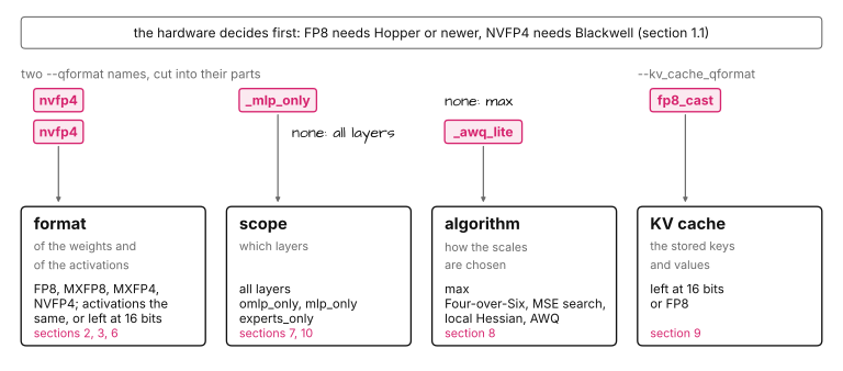
As Figure 2 shows, a name starts with the format, and a scope or an algorithm follows if it differs from the default, which is all layers and an algorithm called max. My runs mostly used these names (the YAML above is what nvfp4_mlp_only with --kv_cache_qformat fp8_cast stands for), so I will mention the name whenever it helps to find a configuration again.

1.3 The Words in the Fields#

The fields refer to parts of the model, so let’s name those first.

Almost all weights of a language model sit in linear layers, each of which multiplies a weight matrix by its input. The input is not known in advance, since it depends on the text. To keep the two apart, these run-time values are called activations. A format can apply to the weights alone or to both, which is often written as a pair: W4A4 means 4-bit weights and 4-bit activations, and W4A16 means 4-bit weights with activations left at 16 bits.

Every layer of the model has two modules. The attention module has three linear layers that turn each token into a query, a key, and a value, or q, k, and v for short, and a fourth one, the output projection. The MLP module has three more, called the gate, the up, and the down projection. In a Mixture-of-Experts (MoE) model, the MLP is replaced by many small MLPs called experts, of which only a few are used for each token. The scopes in a recipe are named after these parts: mlp_only, for example, leaves the attention module alone.

The KV cache belongs to the attention module. To produce the next token, attention compares the query of the current token with the keys of all earlier tokens and mixes their values accordingly. Since the keys and values of earlier tokens don’t change, the server keeps them in memory instead of computing them again, and this memory is the KV cache. It holds activations, not weights, and it grows with the length of the text and the number of requests.

Two more words come up all the time. Calibration means running a few hundred text samples through the model to see what its activations look like, which is the only data that this kind of quantization needs, since the model is not retrained. And a kernel is the piece of GPU code that carries out one operation, such as multiplying a 4-bit matrix by a 4-bit input.

1.4 A Scale and a Grid#

Now, what does a format do to a number? In BF16, every weight takes 16 bits. With 4 bits per weight, we only have 16 different codes, so the first thing to decide is which 16 numbers those codes stand for. This fixed list of numbers is called the grid. NVFP4 uses a tiny floating-point format for it, with 1 sign bit, 2 exponent bits, and 1 mantissa bit (E2M1 for short). Its values are 0, 0.5, 1, 1.5, 2, 3, 4, and 6, plus their negatives, 15 in all.

The weights of a model are nowhere near these values. Let’s take 16 neighboring weights from the first MLP layer of Qwen3-8B. The largest of them is 0.040 in absolute value, and a typical one is 0.015. To get them onto the grid, we divide all 16 by a common number, the scale, which we choose so that the largest weight lands on the largest grid value: 0.040 / 6 = 0.00667.

After dividing, we round each weight to the nearest grid value. The first weight, -0.0238, becomes -3.57 and is stored as -4. What ends up in the file are the 16 codes and the scale. To get a weight back, we multiply its grid value by the scale, which gives -0.0267 here instead of the original -0.0238. Figure 3 below shows this for all 16 weights.

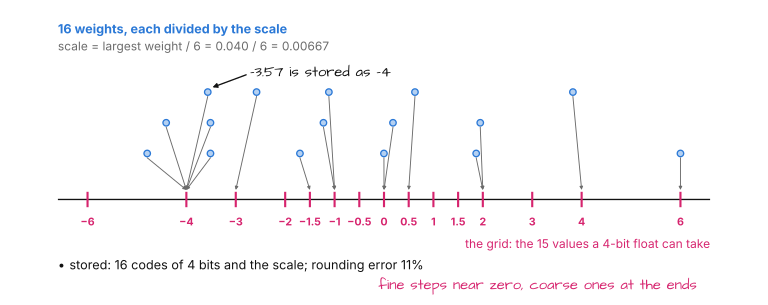
In Figure 3, the grid has small steps near zero and large steps at the ends, which fits weights reasonably well, since most of them are small. The rounding still costs precision: if we treat the 16 weights as a vector, the error is 11% of its length. I will use this measure, the length of the error divided by the length of the vector, as the rounding error throughout the article.

Taking the scale from the largest value is the recipe’s default algorithm, max. FP8 works the same way with a larger grid of 4 exponent bits and 3 mantissa bits (E4M3), whose values reach 448. So, this is all a quantizer stores: codes on a fixed grid, and a scale.

1.5 How I Measured#

All the numbers in this article come from the following setup, and its limits apply everywhere, so I state them once.

I ran almost every configuration once, with the unmodified hf_ptq.py and 512 calibration samples of up to 512 tokens from the CNN/DailyMail dataset, on Qwen3-8B, which has 36 layers. (GB means 10⁹ bytes.)

For accuracy, the first measure is the perplexity on the WikiText-2 test set, which says how well the model predicts each next word and is 9.73 for the original. I computed it on ModelOpt’s simulation of the format before the file is written, in which every quantized value is converted straight back to 16 bits. One repeated run gave the same number to all digits, and fewer calibration samples moved it by 0.01 at most. But the simulation has a quirk: whenever I quantized one more thing to FP8 in a configuration (the KV cache, for example), its perplexity went down, five times out of five and by up to 0.05. So, I ignore differences below 0.05.

The second measure is GSM8K: 1,314 grade-school math problems per served checkpoint, run through SGLang with thinking off and at most 512 output tokens. The original solved 91.3%. One score has a standard error of 0.8 points, a difference between two scores has 1.1, and I scored no checkpoint twice. Eight variants of NVFP4 on all layers that differ only in the algorithm or the input scale of section 3 scored between 89.8% and 92.6%. The 4-bit checkpoints also wrote longer answers, 155 to 182 tokens on average against 140 for the original, which neither measure counts. I therefore rest the claims about formats, scopes, and algorithms on the perplexity and don’t read a single GSM8K difference of two or three points as a result. The one place where I do use GSM8K is the KV cache, for reasons that section 9 gives.

For speed, I served each checkpoint with SGLang on one B300 and sent requests with 1,024 input tokens of real conversation text and a forced length of 256 output tokens, at 1, 16, and 128 concurrent requests, three times each. Because prompts repeat between these levels, SGLang could reuse 6% to 25% of the input tokens, equally for every checkpoint. Most Qwen3-8B runs shared one GPU, one after another. A second round on another B300 repeated NVFP4 on all layers (within 2% of the first), mlp_only, and AWQ, and added the KV cache on all layers. For AWQ (Figure 1) and for all layers with the KV cache (Figures 1 and 9), the throughput comes from this round.

2. The Number Format#

The format is the field that decides how many bits a weight takes, and the main question behind it is how many weights can share one scale.

2.1 Who Shares a Scale#

In section 1.4, our 16 weights shared one scale. But the scale has to be stored as well, so the more weights share one, the cheaper it gets. Why not use a single scale for a whole weight matrix, then?

For FP8, that is what the preset fp8 does, and it works because an 8-bit float keeps about the same relative precision for small and large values. I quantized all 6.95 billion weights in the linear layers of Qwen3-8B this way with ModelOpt’s own code, and the rounding error was 2.65% with one scale per matrix and 2.64% with one scale per row.

With 4 bits, this no longer works. The matrix that our 16 weights come from has 12,288 rows and 4,096 columns. Its largest weight is 0.59, whereas a typical weight is 0.016. If the scale has to make room for the 0.59, a typical weight sits at 3% of the maximum, and a grid of 15 values has almost nothing down there. I tested this with a 4-bit integer grid, which is the usual choice when a whole matrix shares one scale: almost every weight was stored as -1, 0, or 1, and the rounding error over all layers was 87.5%.

The way out is to let fewer weights share a scale. The largest weight in the row of our example is 0.089, and the largest among our 16 weights is 0.040, so the smaller the group, the closer its scale is to what its weights need. A format that gives every small group its own scale is called a block format, and the group is called a block. ModelOpt has two families of them, and they differ in what the scale of a block looks like.

2.2 MX: A Power of Two for Every 32 Values#

The MX formats (short for microscaling) come from an open standard. A block has 32 values, and its scale is a power of two, so only its 8-bit exponent is stored. Spread over 32 values, that’s a quarter of a bit per value, so MXFP8 costs 8.25 bits per value and MXFP4 costs 4.25.

A power of two is cheap to store and to multiply by, but it is a coarse choice. ModelOpt rounds the scale up to the next power of two, which can be almost twice as large as needed. For the first 32 weights in our row, the largest weight lands on 4.03 instead of 6, so the top of the grid goes unused.

2.3 NVFP4: An FP8 Scale for Every 16 Values#

NVFP4 is NVIDIA’s 4-bit format, and it makes two changes. A block has 16 values instead of 32, the recipe’s block_sizes, and its scale is an FP8 number instead of a power of two (scale_bits: e4m3). One FP8 scale for 16 values adds half a bit per value, which makes 4.5 bits per weight.

The complication is that an FP8 number is itself a small float. It can’t go above 448, and below 1/64, which is about 0.016, it loses precision. The scale that our block needs, 0.00667, is already below that. That’s why NVFP4 has a second scale, one for the whole matrix, and stores each block scale as a multiple of it. I will call the two the block scale and the tensor scale. ModelOpt sets the tensor scale to the largest weight of the matrix divided by 6 × 448, so that the block containing this weight gets exactly 448, the largest multiple that FP8 can express.

Let’s work this out for our block. The largest weight of the matrix is 0.59, so the tensor scale is 0.59 / 2,688 = 0.000219. Our block needs a scale of 0.00667, which is 30.4 times the tensor scale. However, FP8 has 3 mantissa bits, so around 30, it can only express even numbers: 28, 30, 32. ModelOpt stores 30, the nearest one. As a result, the largest weight of the block lands on 6.08 instead of 6 and is stored as 6. Figure 4 below shows what is stored for one row of the matrix.

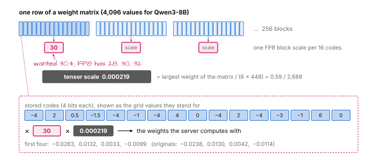
Because the block scale in Figure 4 is 30 instead of 30.4, our first weight comes back as -0.0263 where section 1.4 had -0.0267. We will come back to this 30 in section 8, because nothing forces us to store the nearest value.

2.4 What the Format Costs#

Now, how much precision do we lose with each of these formats? Figure 5 below puts the first 32 weights of our row through three of them.

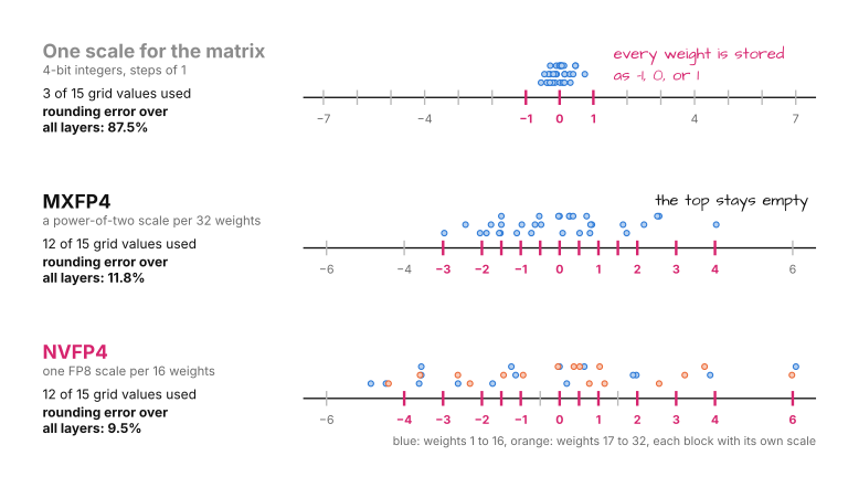
At the top of Figure 5, we see the failure from section 2.1 again, with only 3 of the 15 grid values in use. MXFP4 in the middle uses 12 of them but leaves the top of the grid empty because of its power-of-two scale. NVFP4 at the bottom also uses 12 and includes the top. Over all layers, the rounding error is 11.8% for MXFP4 and 9.5% for NVFP4.

A rounding error on the weights is not yet a loss in accuracy, though, so I also measured the perplexity of each format with both weights and activations quantized. Figure 6 below shows it against the size of the checkpoint.

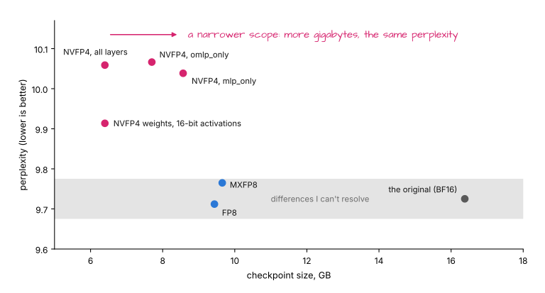
In Figure 6, FP8 and MXFP8 both sit inside the gray band, at 9.71 and 9.77 against 9.73 for the original. So, on this model, 8 bits cost nothing that I can measure and take the file from 16.4 GB to 9.4 GB. The 4-bit points sit clearly above the band. NVFP4 on all layers is at 10.06 and 6.4 GB. MXFP4, which I left out of the figure, was at 10.92, more than three times the loss of NVFP4 for a rounding error that is only a quarter larger. Its activations use the coarser blocks as well, which is probably part of the reason.

Figure 6 also has points that we haven’t discussed yet: NVFP4 with fewer layers quantized, which sit to the right of the full one at the same height, and NVFP4 with 16-bit activations, which sits lower. They belong to sections 7 and 6.

The format field decides between three levels. FP8 costs no measurable accuracy on this model, NVFP4 costs a third of a point of perplexity for a file of 39% of the original size, and MXFP4 costs much more for almost the same size.

3. Activations#

The format field has a second half, the input_quantizer. In a W4A4 recipe, the input of each linear layer is quantized to NVFP4 as well, with the same layout as the weights. But there is an obvious problem: when we produce the checkpoint, the activations don’t exist yet.

3.1 What Can Be Stored in Advance#

The block scales depend on the values of each block, so the server has to compute them in every forward pass, from the largest value in each block of 16.

What can be stored is the tensor scale, and this is what calibration is for. ModelOpt runs the calibration samples through the model once and records, for the input of each linear layer, the largest value it has seen. The stored number is this value divided by 6 × 448, and it is called the input scale.

3.2 The Window#

This one number matters more than it seems, because the block scales are expressed as multiples of it, and such a multiple has to fit into an FP8 number. At the upper end, FP8 stops at 448. At the lower end, it keeps its full precision down to 1/64, gets coarser below that, and ends at 1/512.

In other words, the input scale places a window. A block of activations can be represented well if its largest value lies between 0.09 and 2,688 times the input scale (that’s 6/64 and 6 × 448), which is about four and a half orders of magnitude. To see what happens outside, I fed made-up blocks of random values to the function that SGLang calls to quantize activations. The upper part of Figure 7 below shows the result.

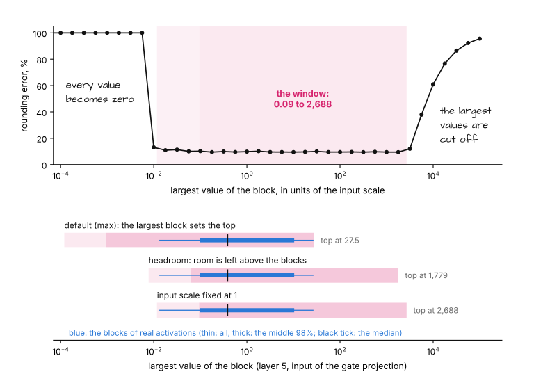
In the upper part of Figure 7, the rounding error stays at about 10% across the window and across the light part below it. Below 0.006 times the input scale, every value of a block comes back as zero. And above 2,688, the largest values of a block are cut off at the top of the grid, so the error climbs to 61% at 10,000.

The lower part of Figure 7 shows real activations for comparison. At the input of one MLP layer of Qwen3-8B, the largest values of the blocks range from 0.01 to 27. That’s roughly three orders of magnitude, so they fit into the window with room to spare, and the question is only where to put it.

3.3 Where to Put the Window#

ModelOpt has three answers, which are the three rows at the bottom of Figure 7. The default takes the largest value seen during calibration as the top of the window. A second policy, nvfp4_act_headroom (added in August 2026), places the small blocks near the bottom and leaves the room above them free for values that calibration didn’t see. And a third one doesn’t look at any data and sets the input scale to the constant 1.

On Qwen3-8B, the choice made no difference that I could measure. With all layers in NVFP4, the perplexity was 10.06 with the default, 10.06 with headroom, and 10.05 with the constant. When I captured the inputs of all 252 quantized linear layers on other text, the median layer had a rounding error of 9.0% under all three. Only at a handful of inputs did headroom or the constant cut off or zero values that the default kept. So, I stayed with the default.

3.4 What 4-Bit Activations Cost#

The number that matters more is what 4-bit activations cost. With NVFP4 weights and 16-bit activations, the perplexity of Qwen3-8B was 9.91, and with NVFP4 activations on top, it was 10.06. Of the 0.33 that NVFP4 loses against the original, 0.15 comes from the activations, almost as much as from the weights.

This is easy to overlook, since the activations take no space in the file. But it means that almost half of the accuracy price of NVFP4 is paid for something that makes the checkpoint no smaller. What it buys is speed, and we will see how much in sections 5 and 6.

3.5 One Whole Layer#

We now have every number that an NVFP4 layer uses, so we can write the layer down once and then see where it sits in the model. For an input x in BF16 and a weight matrix W, a quantized linear layer computes the following:

Linear_NVFP4(x, W) = alpha * ( (x_code * s_x) @ (W_code * s_w)^T )   in BF16

  x_code = round_G( x / (s_in * s_x) )              4-bit codes of the input
  s_x    = FP8( max|x| in the block / (6 * s_in) )  one per 16 values
  alpha  = s_in * s_tensor                          one FP32 number

Here, W_code and s_w are the stored codes and block scales of the weights, and s_tensor is their tensor scale. s_in is the input scale from calibration. s_x is the block scale of the input, which the server computes for every 16 values of every input and which is itself an FP8 number, hence the window of section 3.2. round_G rounds to the 4-bit grid, * multiplies each code by the scale of its block, and @ is the matrix multiplication, whose kernel reads the 4-bit codes and their scales and adds up the products in 32 bits. Since the block scales are relative to the tensor scale and the input scale, these two are multiplied back once, as alpha. For our block of weights, a code of -4 with s_w = 30 and s_tensor = 0.000219 gives the -0.0263 of section 2.3.

Figure 8 below shows where this operator sits in one layer of Qwen3-8B.

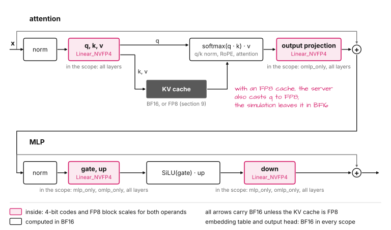
In Figure 8, every arrow carries BF16 as long as the KV cache does. The normalization, the attention itself, the activation function of the MLP, and the additions all work on these values, and 4-bit numbers only exist inside the pink boxes, where an input is quantized, multiplied, and returned in BF16. A server may merge boxes that share an input: SGLang loads q, k, and v as one matrix and gate and up as another, each with one input scale and one tensor scale. ModelOpt’s export gives the merged parts common scales for that purpose.

The figure also shows where each field of the recipe acts. The format decides the grids inside a pink box, the scope decides which boxes are pink, and the algorithm decides how s_w and the codes are chosen. The KV cache is the one box in the attention half that can hold a second format.

4. What Is in the File#

With both halves of the format in place, we can produce a checkpoint and look inside. Below is, in essence, the command that I ran for NVFP4 on the MLP layers with an FP8 KV cache, in the legacy spelling (most other runs passed --kv_cache_qformat none; without the flag, the script adds this KV cache):

python hf_ptq.py \
  --pyt_ckpt_path Qwen/Qwen3-8B \
  --qformat nvfp4_mlp_only \
  --kv_cache_qformat fp8_cast \
  --dataset cnn_dailymail \
  --calib_size 512 \
  --export_path ./Qwen3-8B-NVFP4

The new spelling, which I didn’t run, replaces the two format flags with --recipe general/ptq/nvfp4_mlp_only-kv_fp8_cast. On one B300, the whole run took about 36 seconds, of which the calibration was 6. So, a first attempt at quantizing a model of this size is a matter of seconds.

In the resulting directory, each quantized layer has a small group of tensors in place of its single weight tensor. For the matrix that our 16 weights come from, these are:

mlp.gate_proj.weight           uint8   [12288, 2048]   two 4-bit codes per byte
mlp.gate_proj.weight_scale     FP8     [12288, 256]    one block scale per 16 codes
mlp.gate_proj.weight_scale_2   FP32    one number      the tensor scale
mlp.gate_proj.input_scale      FP32    one number      the input scale

These are exactly the numbers from sections 2 and 3: the codes, the block scales, the tensor scale, and, for the activations, the one number that calibration recorded. The script also writes a small file, hf_quant_config.json, which tells a server how to read the tensors:

{
  "producer": {"name": "modelopt", "version": "0.47.0"},
  "quantization": {
    "quant_algo": "NVFP4",
    "kv_cache_quant_algo": "FP8",
    "group_size": 16,
    "exclude_modules": ["lm_head", "model.embed_tokens", "model.layers.0.self_attn*", "..."]
  }
}

The list exclude_modules names every layer that was left in BF16, and two entries in it are there for every scope: the embedding table at the input of the model and the output head at its end. They are worth a second look, because they explain the size of the file. With all layers in NVFP4, the checkpoint of Qwen3-8B is 6.4 GB, and these two tensors, with 1.24 billion parameters in BF16, are 2.5 GB of it, or 39%. Quantizing the output head alone would save another 0.9 GB. These two tensors are why the file is 2.6 times smaller than the original and not the 3.6 times that 16 bits against 4.5 bits would suggest.

5. Speed: What the Server Runs#

So far, the format has only made the file smaller. To see why it also makes the model faster, we have to look at what a server does with the four tensors.

5.1 The Two Kernels#

Serving the checkpoint with SGLang takes no special flags, since SGLang reads hf_quant_config.json and picks an implementation for each linear layer by itself:

python -m sglang.launch_server --model-path ./Qwen3-8B-NVFP4 --port 30000

For an NVFP4 layer, this implementation is the operator from section 3.5, in two kernels. A first kernel takes the BF16 input, computes its block scales, and writes out the 4-bit codes, and a second one multiplies the two 4-bit operands, applies alpha, and returns BF16. Below is a simplified excerpt from SGLang:

# Simplified from ModelOptFp4LinearMethod
# once, after loading:
alpha = input_scale * weight_scale_2

# for every forward pass (x is BF16):
x_fp4, x_scale = fp4_quantize(x, 1 / input_scale)  # computes the block scales
out = fp4_gemm(x_fp4, weight, x_scale, weight_scale, alpha)

Compared to the original, the server has one more step per layer, quantizing the input, and in return, the multiplication reads 4.5 bits per weight where it used to read 16.

5.2 What the Format Buys#

Figure 9 below shows the output throughput of Qwen3-8B in each format, relative to the original.

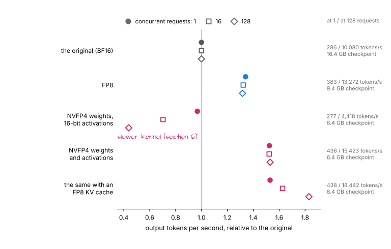
In Figure 9, FP8 is about a third faster than the original at all three loads, and NVFP4 with 4-bit activations is faster again, by another 14% to 16%, which makes 52% over the original. The time until the first token of a long prompt of 8,192 tokens improved as well, from 101 ms for the original to 69 ms with FP8 and 54 ms with NVFP4.

Why is a smaller format faster, even for a single request, where the GPU is far from busy? To produce one token, the model has to go through all of its layers once, and for that, the GPU has to read every weight from its memory once. On a model of this size, that reading takes a large part of each step. So, given a fast kernel, the time per token follows the bytes of weights, on top of a fixed part.

The measurements fit this closely. At one request, a token took 3.44 ms with the original, 2.56 ms with FP8, and 2.25 ms with NVFP4. The weights that a step reads are about 15, 8, and 5 GB (the files without the embedding table, of which only a few rows are read). A fixed 1.6 ms plus 0.12 ms per GB reproduces all three, and NVFP4 with a narrower scope as well, to within 0.05 ms. The fixed part also explains why NVFP4 gains only 14% over FP8 with a third fewer bytes: at 2.25 ms, most of the step is already the part that doesn’t shrink.

6. The Activation Trade-Off#

In section 3.4, we saw that 4-bit activations cost almost as much accuracy as 4-bit weights and make the file no smaller. An obvious idea is to keep the NVFP4 weights and leave the activations at 16 bits. ModelOpt has a preset for that, w4a16_nvfp4, and by perplexity, it is the best 4-bit configuration that I measured, at 9.91 against 10.06.

By speed, it is the worst. In the third row of Figure 9, the weight-only checkpoint is slightly slower than the original for a single request and drops to 70% of the original at 16 requests and to 44% at 128. The file is as small as the full NVFP4 one, and the model is slower than if we had not quantized it at all.

The reason is the kernel. The NVFP4 multiplication that a Blackwell GPU has in hardware needs both operands in 4 bits. For a checkpoint with 16-bit activations, SGLang therefore uses a different kernel, called Marlin, which is the same one that it falls back to on GPUs before Blackwell. Marlin reads the 4-bit weights, but it converts them back to 16 bits and multiplies there, which evidently costs more than the smaller weights save.

The numbers show where the time goes. During generation, a token took 3.44 ms at one request, the same as with the original, so the smaller weights bought nothing. And the first token of a 1,024-token prompt took 48 ms where the original needed 16, so processing the prompt, where many tokens are multiplied at once, was three times slower. With more requests, more of the work looks like that.

ModelOpt’s recipe guide recommends weight-only quantization for deployments with few requests at a time, such as edge devices, where “shrinking weights is the main win”, and I measured no such device. For data-center serving, the guide prefers quantized activations too and notes that the Marlin fallback of another engine “measured slower than BF16”. With SGLang on a B300, weight-only was slower than the original at every load. On Blackwell, the precision of the activations decides whether the fast kernel runs at all, which makes it the half of the format that sets the speed.

7. Scope#

The scope is the field that says which layers get the format. With the default, every linear layer except the output head is quantized, and the README of the script advises against that for NVFP4:

For NVFP4 quantization specifically, we recommend nvfp4_mlp_only, nvfp4_experts_only, or nvfp4_omlp_only to achieve higher accuracy by restricting quantization to the MLP/expert layers (and optionally the o_proj layer) while keeping the attention QKV projections unquantized.

The three scopes in the quote are narrower steps of the same idea. The gray labels in Figure 8 show two of them: mlp_only quantizes the two boxes of the MLP, and omlp_only adds the output projection, but not q, k, and v. experts_only is for MoE models and only quantizes the experts.

On Qwen3-8B, I could not measure the gain that the README promises. The three points at the top of Figure 6 in section 2.4 show this: the perplexity was 10.06 with all layers, 10.07 with omlp_only, and 10.04 with mlp_only. Nearly all of the loss comes from the MLP, so taking the attention module out of the scope removes very little of it.

What the narrower scope does change is everything else. The attention projections stay at 16 bits, so with mlp_only, the checkpoint grew from 6.4 GB to 8.6 GB. By the reasoning of section 5.2, more bytes per step mean a slower model, and it was 8% to 9% slower than with all layers at every load.

Section 10 has a model on which the scope did make a difference. On Qwen3-8B, which has no experts, the narrower scope cost size and speed and bought no accuracy that I could measure.

8. The Calibration Algorithm#

The algorithm is the last of the three fields that a legacy name sets, and it is where ModelOpt offers the most choice. Figure 10 below shows the perplexity of Qwen3-8B, with all layers in NVFP4, for the default and four alternatives.

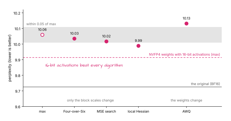
In Figure 10, two of the four alternatives are inside the band around the default. The other two, both explained below, sit just outside it, at 9.99 and 10.13. The dashed line for 16-bit activations is lower than all of them. So, these five move the result by less than the single decision about the activations. To see why, it helps to look at what these algorithms are free to change.

8.1 A Better Block Scale#

In section 2.3, our block wanted a scale of 30.4 times the tensor scale, and max stored 30, the nearest value that FP8 offers. But a block scale is an 8-bit number that we choose once and offline, so we can also try every value. An FP8 number has 126 values that are positive and finite, and for each of these, we can quantize the block and measure the rounding error. Figure 11 below shows the result for our block.

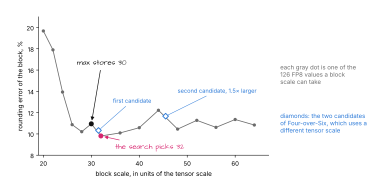
In Figure 11, the error at 30 is 10.9%, and the next candidate, 32, brings it down to 9.8%. With 32, the largest weight sits at 5.70 and is still stored as 6, but several of the smaller weights land closer to a grid value.

Three of the algorithms are variants of this search. The MSE search (the preset nvfp4_w4a4_weight_mse_fp8_sweep) does exactly what we just did, for every block. Four-over-Six only tries two candidates, the scale that puts the largest weight on 6 and one that puts it on 4, which are the diamonds in Figure 11. And the local Hessian runs the full search but scores a candidate by the error in the output of the layer. For that, it records the sizes and correlations of each block’s 16 inputs in one more calibration pass.

Over all layers, these searches lowered the rounding error of the weights from 9.5% to 8.7% with Four-over-Six and to 8.1% with the MSE search. That is a real improvement in the weights. But it only acts on the weights’ share of the loss, which section 3.4 put at a little more than half, and it starts from a format that already gives every 16 weights a scale of their own. The best of the searches, the local Hessian, recovered 0.07 of the 0.33. That is over a third of the weights’ share, which is all that a scale can reach.

8.2 Changing the Weights#

AWQ, short for activation-aware weight quantization, goes further and changes the weights before rounding. It multiplies each column of a weight matrix by a factor and divides the matching input by the same factor, so that columns with large inputs take up more of the grid. Where the division can’t be folded into a neighboring layer, the factor stays in the checkpoint as an extra tensor, and the server applies it at run time.

On Qwen3-8B with NVFP4, AWQ didn’t lower the perplexity: it was 10.13 against 10.06. When I served it back to back with a repeat of the default on the same GPU, it was also 7% slower at one request and 12% slower at 128. It was not broken: on a 4-bit integer grid with one scale per 128 weights, the kind of format that it was designed for, the same code improved the perplexity from 10.40 to 10.25. It seems that NVIDIA doesn’t use it for NVFP4 either. Among ModelOpt’s model-specific NVFP4 recipes, aliases aside, I counted 18 with max, 10 with the MSE search or Four-over-Six, 1 with the local Hessian, and none with AWQ.

So, for NVFP4, I would treat the algorithm as the last field to touch. The searches are cheap, about a minute of extra work on this model, and the local Hessian is the one I would try if the accuracy fell short. But none of them changes what kind of result we get.

9. The KV Cache#

The fourth field is separate from the other three, because it doesn’t concern the weights at all. As section 1.3 described, the KV cache is where the server keeps the keys and values of earlier tokens, and by default, they are stored in 16 bits like every other activation.

The entry in the recipe changes that to FP8. With the legacy flags, the script adds it by default, so a checkpoint requests an FP8 KV cache unless we pass --kv_cache_qformat none, as I did for most runs. In the default variant, fp8_cast, nothing is calibrated: the scale is fixed at 1, and the server converts each key and value to an 8-bit float when it stores it. ModelOpt writes this request into hf_quant_config.json, as we saw in section 4, and SGLang switches its cache to FP8 when it finds it.

9.1 What It Buys#

For speed, I served NVFP4 with and without an FP8 KV cache, on all layers and with mlp_only. At one request, the cache made no difference beyond the 2% between two runs. At 16 requests, it added up to 6%, and at 128, about 20% for both. All layers with an FP8 KV cache, the last row of Figure 9, was the fastest configuration that I measured, at 18,442 tokens per second.

This fits the picture from section 5.2. A decoding step has to read the weights once, but it also has to read the keys and values of all tokens of all running requests. In BF16, one token of Qwen3-8B takes 147 kB of KV cache. With a single request of about a thousand tokens, that is nothing next to 5 GB of weights. With 128 such requests, it is roughly 22 GB per step, four times the weights, and halving it is the largest saving left. In FP8, the same memory also holds twice as many tokens.

9.2 What It Costs#

By the perplexity, the cache cost nothing: the simulation gave 10.02 with it and 10.06 without it. ModelOpt’s guide calls fp8_cast “the safe default”.

GSM8K says something else. With all layers in NVFP4, the score went from 92.6% to 89.4% when I added the cache, and with mlp_only, from 92.5% to 90.3%. By the rule from section 1.5, one such drop proves little, and the 92.6% is the top of the range that I gave there. But both scopes fell, and there is a reason why the perplexity could have missed it.

The reason is that the perplexity comes from ModelOpt’s simulation, and the simulation and the server don’t do the same thing. The difference is at the arrow labeled q in Figure 8. In the simulation, the preset quantizes the keys and the values on their way into the cache and leaves the query in 16 bits. When the cache is FP8, SGLang’s attention backend on a B300 converts the query to FP8 as well. Both sides of the comparison between a query and a key are then 8-bit in serving and only one of them in the simulation. I have not shown that this is the cause of the drop, but the number that was supposed to approve the KV cache did not measure what the server runs.

So, the KV cache is a trade of its own: a fifth more throughput under heavy load against a risk to accuracy that has to be tested on a task, with the served checkpoint.

10. The MoE Contrast: Qwen3-30B-A3B#

Everything so far was measured on one model of 8 billion parameters, without experts. To see what carries over, I repeated the main steps on one MoE model, Qwen3-30B-A3B-Instruct-2507 (Qwen3-30B-A3B below), in which every layer has 128 experts and uses 8 of them for each token.

Most of the picture is the same. FP8 on all layers moved the perplexity from 7.26 to 7.31. NVFP4 on the experts took it to 7.47, and with 16-bit activations, to 7.38, so the activations again cost about half of the loss. The MSE search gave 7.46, and the three ways to place the window gave 7.47, 7.47, and 7.46. As on the smaller model, the format and the activation precision moved the result, and the algorithm and the placement of the window left it where it was.

MoE models also raise a problem for the one algorithm that helped. The local Hessian needs calibration tokens for every block that it tunes, and with 8 of 128 experts active, an expert sees one token in 16 on average, and a rarely chosen one far fewer. The authors of the algorithm name this as open: “Many experts in a sparse MoE see very little calibration data.”

In serving, the experts-only checkpoint was 12% faster than the original at one request and 64% faster at 128, with the same GSM8K score (95.5% against 95.4%). FP8 on all layers, in contrast, was 13% slower than the original at one request and 12% faster at 128. That says little about the format. SGLang’s log warned that it had no tuned kernel configuration for the experts of this checkpoint. A third-party MXFP8 checkpoint, which ran on the same family of expert kernels as the BF16 and NVFP4 runs, was 10% faster than the original at one request. On this MoE model, the kernel that the experts got mattered more than the bits.

The scope is where this model differs. With experts_only, the checkpoint shrank from 61.1 GB to 19.4 GB at a perplexity of 7.47. With all layers in NVFP4, the perplexity rose to 7.61, so here, leaving the attention module out bought 0.14, where on Qwen3-8B it bought nothing. In an MoE model, the experts hold most of the weights anyway, so the narrow scope gives up little size. This is one model, but on it, the README’s advice held.

11. What Went Wrong, and What I Left Out#

Three things went wrong along the way that a reader who follows the same path may run into. The scope patterns of a recipe are matched against layer names, and a pattern that matches fewer layers than intended goes through without an error, so it is worth reading exclude_modules after every run. A checkpoint in which I mixed NVFP4 for the MLP with FP8 for the attention module was written without complaint and then failed to load in SGLang, with an error about a missing input scale. And the script still prints a warning that SGLang can’t load the weight-only checkpoint, which is no longer true.

I also left several things out:

• GPTQ and SVDQuant, two more algorithms that change the weights. GPTQ took 31 minutes and ended at a perplexity of 10.25, worse than max, and SGLang doesn’t load SVDQuant checkpoints.
• The integer and GGML formats among the presets, since SGLang doesn’t load ModelOpt checkpoints in them.
• AutoQuantize, a search that picks a format per layer for a given budget of bits.
• Quantization-aware training and distillation, which ModelOpt offers for the cases where quantization after training loses too much.
• Other engines. The checkpoint format is meant to be loaded by TensorRT-LLM and vLLM as well, but I only tested SGLang.
• 8-bit activations with 4-bit weights (the w4a8 presets), which I didn’t run.
• GPUs before Blackwell, for which I have no measurements.

12. Conclusion#

For a model like Qwen3-8B, I would quantize all layers, with NVFP4 for weights and activations on a Blackwell GPU (the preset nvfp4 with --kv_cache_qformat none) and with FP8 on a Hopper GPU. I would leave the algorithm at max and add the FP8 KV cache only for heavy load, and only after testing it on a task.

Let’s go through the fields once more with Figure 1 in mind, since each of these choices follows from one of its rows or columns.

The format. This is the field that decides what we get. FP8 gave a third more speed and 58% of the size for no measurable loss. NVFP4 gave 52% more speed and 39% of the size for 0.33 of perplexity. The activations belong to this decision: leaving them at 16 bits recovered almost half of the loss and made the model slower than the original, because the fast kernel needs both operands in 4 bits. So, with SGLang on Blackwell, I would serve FP8 before weight-only NVFP4.

The scope. On Qwen3-8B, I would quantize all layers. With mlp_only, the file was 2.2 GB larger and the model 8% to 9% slower for the same perplexity.

The algorithm. I would start with max and try the local Hessian only if the accuracy fell short. It was the best of the five in Figure 10 and recovered a fifth of the loss, which is barely more than I can resolve.

The KV cache. I would leave it at 16 bits until a task benchmark on the served checkpoint says that FP8 is safe for the model in question, and then use it where many requests run at once.

Two of these choices go against ModelOpt’s guide: all layers as the scope, and a 16-bit KV cache. The guide says to begin with the narrowest scope and to widen it only as needed, and it calls fp8_cast the safe default for the KV cache, though the script’s README says to disable it if the accuracy falls short. On the other two fields, we agree: quantize the activations for a server, and start with max. On Qwen3-8B, the narrowest scope protected nothing that my two measures can show, and GSM8K fell in both runs with the KV cache.

Still, I don’t think that the guide is wrong. For a model without experts, it also offers a middle way, FP8 for the attention module, which I couldn’t test in serving since SGLang failed to load that mix. And the one MoE model that I measured agreed with it on the scope. So, for a large MoE model, I would follow the guide on the scope, and for a model like Qwen3-8B, I would measure both scopes before choosing the narrow one.

What I would take to another model is the order of the questions. The hardware limits the format, and the format and its activations set the size, the speed, and most of the accuracy. A run with one of the five algorithms takes at most two minutes on Qwen3-8B, so I would measure the rest instead of guessing.