How a Row Meets Its Experts

Several of the largest open-weight models are Mixture-of-Experts (MoE) models. Such a model is usually said to have hundreds of billions of weights and to use a few percent of them per token. GLM-5.3 from Z.ai, for example, has 256 experts in each of its MoE layers, and a token goes through 8 of them.

That holds for one token, but a server processes many tokens at once. Suppose I serve 64 concurrent requests with GLM-5.3 on 8 GPUs. One decode step produces one token per request, so it processes 64 tokens. Each token picks 8 experts, which gives 512 picks. When I recorded which experts the model picked in 300 such steps, an average step touched 72% of a layer’s 256 experts, and the busiest expert of a layer got 17 of the 512 picks. A single decode step therefore needs most of a layer’s 4.83 GB of expert weights, and it uses each touched expert for fewer than 3 tokens on average.

The experts are spread over the 8 GPUs, and so are the tokens. Inside the model, a token is a vector of 6,144 numbers that moves from layer to layer. A batch of tokens is a matrix with one row per token, so I will call a token’s vector a row. This article asks how a row meets its 8 experts when both are spread over several GPUs, and what that costs.

SGLang, the inference engine I use throughout, has five options:

1. Cut every expert into slices and give each GPU one slice of every expert. Every GPU then does part of the work for every row.
2. Leave the experts whole, give each GPU some of them, and put every row on every GPU.
3. Mix the first two: form groups of GPUs that share a set of experts and slice them within the group.
4. Leave the experts whole and let each row travel to the GPUs that hold its experts.
5. Leave the rows where they are and let the weights travel to them.

A server doesn’t have to use one option for all of its work. Processing a prompt, called prefill, handles thousands of tokens at once. Generating, called decoding, handles one token per request. The two are so different that large deployments run them on separate servers: a prefill server hands its result to a decode server. This is called disaggregated serving, and the two kinds of servers can use different numbers of GPUs and different options. I therefore ask the question twice: once for a decode step and once for a chunk of a prompt during prefill.

I describe the mechanisms from the SGLang source code and link to the files along the way. All measurements are for GLM-5.3 with its expert weights stored in NVFP4, NVIDIA’s 4-bit floating-point format. I use MB and GB for powers of 1,000. Every timing ran on one machine with 8 B300 GPUs (NVIDIA’s Blackwell Ultra generation), either on all 8 or on one GPU with the share of the work that one of 8 would have. Everything beyond 8 GPUs is a calculation, and I say so each time.

For the basics of how GPUs exchange data during inference, see How GPUs Talk to Each Other During LLM Inference. You don’t need that article to follow this one.

1. One MoE Layer#

In a standard transformer layer, the attention module is followed by a feed-forward module of two or three large matrices. An MoE layer replaces this module with many smaller ones, called experts, plus a router that chooses among them.

The router is a small matrix that turns a row into one score per expert, so 256 scores in GLM-5.3. The 8 experts with the highest scores process the row, and their outputs are weighted by the scores and summed. GLM-5.3 also has one shared expert per layer that processes every row, whatever the router picks. Figure 1 shows the path of one row.

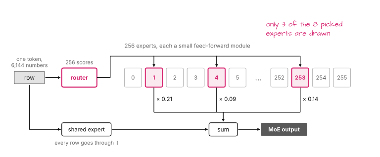
An expert in GLM-5.3 consists of three matrices of 2,048 × 6,144 weights. Two of them map the row to 2,048 numbers each, which are multiplied with each other, and the third maps the product back to 6,144. That makes 37.7 million weights per expert, or 18.9 MB at 4 bits per weight (without the scale factors that NVFP4 stores alongside the 4-bit values). One layer’s 256 experts take 4.83 GB. Of GLM-5.3’s 78 layers, 75 are MoE layers, and their experts take 362 GB together, more than one B300’s 288 GB of memory.

If a batch has T tokens and each token picks 8 of the 256 experts, an expert gets T × 8 / 256 = T / 32 picks on average. With 64 concurrent requests, that’s 2 picks per expert in a decode step, and each pick puts one row on one expert. During prefill, SGLang processes prompts in chunks. In my setup, each of the 8 GPUs processes 1,024 prompt tokens at a time, 8,192 together. I will call that an 8,192-token chunk, and it gives each expert 256 picks on average. Figure 2 shows the batch sizes in between.

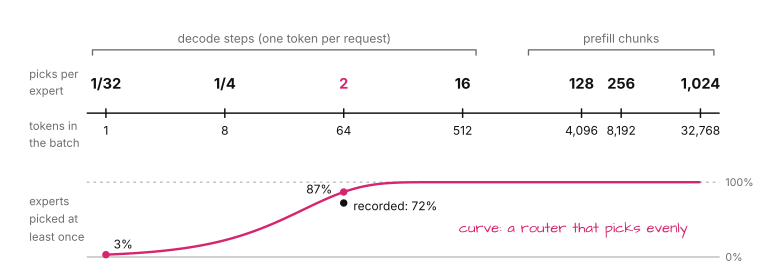
The average hides how unevenly the router picks. A router whose picks are uniformly random, which I will call an even router, would touch 87% of the experts in a 64-token step. My recording shows 72%, because the router favors a few experts. I will call this the router’s skew.

What does it cost to run such a layer for 64 rows?

2. A Decode Step Is Bound by Reading Weights#

To run one row through an expert, a GPU has to read all 18.9 MB of that expert’s weights from memory. The arithmetic, by contrast, grows with the number of rows. With 2 rows per expert, running an expert mostly means reading its weights. The rest of the article builds on this claim: the time the experts take in a decode step is set by the expert weights that are read. What counts is how many experts are touched, not how many rows there are or which GPU gets them.

I ran ShareGPT conversations, a public set of chats, through a GLM-5.3 server. For one MoE layer in the middle of the model, I captured everything that SGLang passes to its expert kernel, the GPU program that runs the experts: the layer’s expert weights, the rows, and the router’s picks.

I replayed these calls on one B300 with the same kernel (from FlashInfer, the kernel library that SGLang uses) and timed them. The GPU held an eighth of every expert, as each of 8 GPUs does under option 1. With NVFP4’s scale factors, those slices total 0.68 GB, which is 21 MB per whole expert and 5.4 GB per layer. I use these sizes from here on. Figure 3 shows the time against batch size.

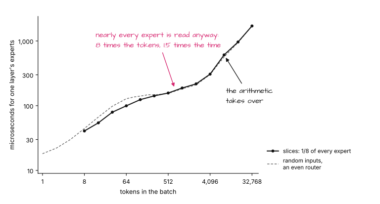
The curve in Figure 3 has three parts. Up to 256 tokens, the time rises from 41 microseconds at 8 tokens to 100 at 64 and 142 at 256, because more tokens touch more experts. Between 256 and 2,048 tokens, the curve is flatter: 8 times the tokens cost 1.5 times the time (218 against 142 microseconds), because nearly all experts are read either way. Beyond 2,048 tokens, the arithmetic dominates, and the time grows with the tokens.

How do we know that reading limits the first two parts? There are three signs. The first is a test kernel that only reads the same 0.68 GB and sums it. It takes 142 microseconds on that GPU, about the time of the expert kernel at 256 tokens, where nearly every expert is touched. The test is a plain sum and not the fastest possible read, so it shows only the order of magnitude. The second is Figure 4, which plots each decode step’s time against the megabytes of expert weights that it reads. For it, I also replayed each step 8 times, once for each GPU of a setup where every GPU holds 32 whole experts instead of slices (section 4.2).

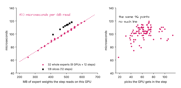
On the left of Figure 4, the magenta points lie on a straight line: 28 microseconds plus 150 for every gigabyte of weights, regardless of which experts are read. The black points for slices lie about 10 microseconds above it. On the right, the same points scatter. Over the 96 points, the correlation between time and picks is 0.34, against 0.998 between time and megabytes.

The third sign is the dashed line in Figure 3. It shows the same kernel with the even router from section 1. Up to about 256 tokens, the even router is slower, because it spreads its picks over more experts and so reads more bytes.

The captured steps have 63 tokens, not 64. The 12 steps in Figure 4 take 113 microseconds on average with slices, and the first of them takes 99, close to the 64-token point in Figure 3. On a server, a decode step with 64 requests costs each GPU 75 layers × 113 microseconds, or about 8.5 milliseconds for the experts, if every layer behaves like this one. In Figure 3, a 128-token batch, which I built by joining consecutive steps of the same requests, takes 24 microseconds more per layer than a 64-token one, about 2 milliseconds per step. A batch of 128 different requests may touch more experts and cost more.

From here on, I use one rule: for a decode step, we count the experts that are touched, and for a prefill chunk, which sits in the third part of Figure 3, we count the rows.

As section 1 showed, the experts don’t fit on one GPU. Rows and experts therefore have to meet across GPUs, and how they meet depends on where a row is when the MoE layer starts.

3. Where a Row Starts#

The attention module, which runs before the MoE layer, determines where a row is. Attention can run on several GPUs in two ways.

With tensor-parallel attention, every matrix of the module is cut into one slice per GPU. All GPUs work on each request together, and afterward each GPU has every token’s row. With data-parallel (DP) attention, each GPU runs the whole attention module, but only for its own share of the requests. Each row is then on one GPU. Figure 5 shows the two cases.

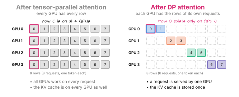
The main reason for DP attention is the KV cache, the memory in which attention keeps what it needs from earlier tokens. GLM-5.3’s attention heads share one set of keys and values, so the cache can’t be split among the GPUs. Tensor-parallel attention stores the KV cache of every request on every GPU, so 8 times on 8 GPUs, whereas DP attention stores it once.

The price is that one request no longer gets all GPUs for its attention. Under the load of section 5.3, with sliced experts, a decode step at 8 concurrent requests takes 7.9 milliseconds with tensor-parallel attention and 13.4 with DP attention. At 256, the order reverses: 37.7 milliseconds with tensor-parallel attention and 24.2 with DP attention.

In SGLang, --tp-size 8 alone selects tensor-parallel attention, and adding --attn-dp-size 8 switches to DP attention on all 8 GPUs. DP attention is the usual choice for throughput, so I use it for all other server measurements.

I will also need three operations, called collectives, in which a group of GPUs exchanges data. In an all-gather, every GPU contributes a piece and ends up with all the pieces. In a reduce-scatter, every GPU contributes a matrix of the same shape, the matrices are summed, and each GPU gets its own part of the sum back. In an all-to-all, every GPU sends a different piece to each of the others. All three finish only when the slowest GPU is done.

With a row on one GPU and its 8 experts somewhere on 8 GPUs, how do they meet?

4. Five Ways for a Row to Meet Its Experts#

Figure 6 shows the five options from the introduction side by side for 8 experts on 4 GPUs.

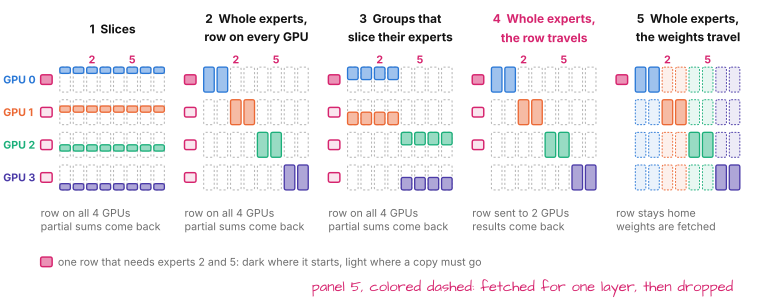
Let’s go through Figure 6 from left to right. In every panel, the four lines of boxes are the 4 GPUs, and a filled box is what a GPU holds of an expert. The square on the left marks each GPU that needs the example row.

4.1 Slices (Option 1)#

By default, SGLang cuts each expert into slices, as it would a feed-forward module. With N GPUs, each GPU gets 1/N of every expert, so with 8 GPUs, each holds a slice with 256 of an expert’s 2,048 intermediate numbers. This is tensor parallelism applied to the MoE layer.

For a given row, each GPU computes an eighth of the expert’s intermediate numbers and multiplies them by its slice of the third matrix. The result has the full 6,144 numbers but is only a partial sum. Adding the 8 partial sums gives the expert’s output.

Every GPU therefore needs every row. With DP attention, an all-gather first copies each row to all GPUs. After the experts, a reduce-scatter adds the partial sums and returns to each GPU the finished rows of its own requests. Figure 7 shows this for 4 GPUs.

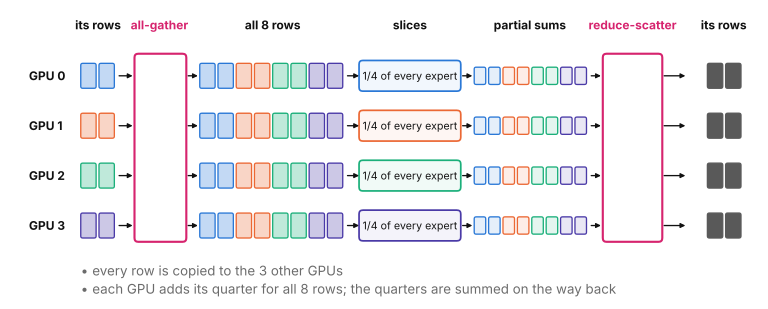
A row is stored as 16-bit floats and takes 6,144 × 2 = 12,288 bytes. On 8 GPUs, the all-gather sends 7 copies of every row, and the reduce-scatter sends 7 partial sums of the same size.

Slices keep the GPUs’ work equal: each does an eighth of every expert for every row. They finish together, whichever experts the router picks. The SGLang cookbook recommends slices (--tp 8 --attn-dp-size 8, where --tp abbreviates --tp-size) as its high-throughput recipe for the NVFP4 version of GLM-5.3 on 8 B300 GPUs.

4.2 Whole Experts (Options 2 and 3)#

The second option, expert parallelism, leaves the experts whole and distributes them. With 8 GPUs, each GPU gets 32 of each layer’s 256 experts.

Each GPU still holds the same share of the layer’s weights, and the router alone decides which experts a step touches. What changes is the work each GPU does. Instead of a narrow slice of every touched expert, a GPU runs each touched expert among its 32 at full width, and only for the rows that picked it. How many picks a GPU gets depends on how popular its experts are.

In SGLang, --ep-size 8 selects whole experts. With that flag alone, SGLang still handles the rows as in Figure 7: every GPU gets every row and skips the picks for experts it doesn’t hold. A reduce-scatter sums the results. Option 3, the mix, also needs every row on every GPU. With --ep-size 4 on 8 GPUs, for example, 4 pairs of GPUs get 64 experts each, and every expert is sliced in two within its pair. I didn’t measure the mix.

4.3 Traveling Rows (Option 4)#

Whole experts don’t need a row on all 8 GPUs, since the row’s 8 experts usually sit on fewer than 8 GPUs. The fourth option sends each row only to the GPUs that hold at least one of its experts.

Traveling takes two steps. In the first, called dispatch, every GPU reads the router’s picks for its own rows and sends each row, together with its picks and scores, to the GPUs that hold the picked experts.

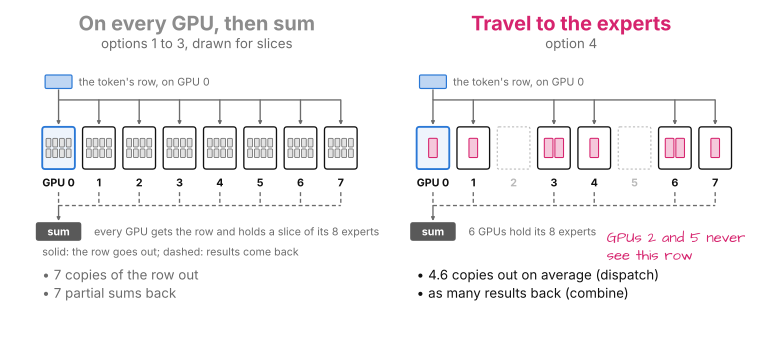
After dispatch, a GPU has a batch of rows from every GPU in the group, and each row needs at least one of that GPU’s experts. The GPU runs its experts on them and weights each output by the router’s score. In the second step, called combine, it sends the results back to the GPUs that the rows came from, and every receiving GPU sums the results per row. Figure 8 shows both steps for one row, next to the row on every GPU.

Both steps are all-to-all operations. Unlike in the all-gather and reduce-scatter of section 4.1, the amount of data one GPU sends to another is not known in advance, since it depends on the router. That is the option’s main difficulty: a GPU’s receive buffers have to be sized for the worst case.

How many GPUs does a row travel to? In my capture, the 8 experts of a row sit on 5.3 of the 8 GPUs on average. For about two-thirds of rows, one of those GPUs is the row’s own. That leaves 4.6 copies to send, whereas slices need 7. An even router gives the same 5.3, which can be calculated. The probability that a GPU holds none of a row’s 8 experts is C(224, 8) / C(256, 8), where C(n, k) is the number of ways to choose k out of n. Summed over the 8 GPUs, that gives 8 × (1 − C(224, 8) / C(256, 8)) = 5.3.

SGLang delegates the two steps to one of several all-to-all backends, which --moe-a2a-backend selects, a2a being short for all-to-all. Its default is none, which keeps every row on every GPU as in options 1 to 3. No GPU backend supports sliced experts, so choosing one sets --ep-size to the number of GPUs. For the measurements, I used the backend from FlashInfer, which calls the same expert kernel through another entry point. Its times are within 3% of the default entry point’s from 32 to 4,096 tokens.

Choosing a backend changes two more settings, and a third can be set by hand.

The first is the format in which the rows travel. The expert kernel for 4-bit weights also takes its input rows at 4 bits per number, so the sender can convert a row before dispatch instead of leaving the conversion to the receiver. A row then takes 3,456 bytes (3,072 bytes of 4-bit values and 384 of scale factors) instead of 12,288. SGLang does this by default for an NVFP4 model, and --flashinfer-a2a-dispatch-type bf16 switches back to 16-bit rows. The results always come back as 16-bit floats.

The second is the shared expert. Every row goes through it, so nothing needs routing. With slices, it is sliced like the other experts. Doing the same with traveling rows would put every row on every GPU again. With a backend selected, SGLang therefore gives every GPU a full copy of the shared expert, and each GPU runs it on its own rows.

In GLM-5.3, the shared expert has the shape of the other experts but is stored in 16 bits. It takes 75 MB, about a ninth of the 0.68 GB of experts per GPU per layer. Over 75 layers, the copies take about 5.7 GB per GPU, 5 GB more than the slices they replace, and the KV cache of my servers shrank by 4%.

The third is the dense layers. GLM-5.3’s first 3 layers have an ordinary feed-forward module instead of experts. Each has three matrices of 12,288 × 6,144 weights, which this checkpoint stores at 8 bits per weight, so a layer takes 226 MB. These modules stay sliced, with an all-gather before and a reduce-scatter after, unless --moe-dense-tp-size 1 asks for copies. With copies of the shared expert and the dense layers, a row leaves its GPU only in MoE layers and only to visit its experts.

4.4 Traveling Weights (Option 5)#

The fifth option reverses the fourth. Distributed Weight Data Parallelism (DWDP), which NVIDIA described in a paper and which SGLang implements, leaves every row where it is and brings the weights to it.

Each GPU still holds only its own 32 experts per layer. Before an MoE layer, it copies the remaining 224 experts of that layer from the other GPUs into a buffer and then runs the layer for its own rows. The copies are plain reads from another GPU’s memory. They run concurrently with the computation and start two layers ahead. No collective is needed, and no GPU waits for another’s computation.

The cost is the amount of data. For GLM-5.3 on 8 GPUs, each GPU would copy 7/8 of a layer’s 5.4 GB, or about 4.8 GB, for every layer of every forward pass. Copying pays off only if the computation takes longer than the copies. The paper uses DeepSeek-R1 on a GB200 rack and puts the break-even for a single request between 8,000 and 16,000 prompt tokens. The computation takes 0.6 times as long as the copies at 8,000 tokens and 1.5 times as long at 16,000.

In a 64-token decode step, a GPU would copy 4.8 GB per layer to run its 8 rows. SGLang prints a warning if DWDP is enabled on a server that also decodes.

In SGLang, DWDP supports one model family (gpt-oss), and support for a second is an open pull request. DWDP doesn’t cover GLM-5.3, so I couldn’t measure this option. The pull request that added DWDP reports that prefill is 1.16 to 1.92 times as fast as with option 2, for gpt-oss-120b on 4 B200 GPUs. The flag is --dwdp-size. The measurements that follow cover options 1, 2, and 4.

To summarize for 8 GPUs, options 1 to 3 send 7 copies of every row, traveling rows send 4.6, and traveling weights send no rows but 4.8 GB of weights per GPU per layer. What does each cost in a decode step?

5. Decode on 8 GPUs#

The three measured options hold the same 0.68 GB of experts per GPU per layer, and a step touches the same experts under all three, so every option reads the same bytes. Up to 64 concurrent requests, they cost about the same, and how evenly the picks fall on the GPUs matters little.

5.1 The Kernel#

I repeated the replay of section 2 with whole experts. Since the 8 GPUs now hold different experts and get different picks, I replayed each GPU’s share on the same B300. Each GPU gets every row, as in option 2. With traveling rows, it would get about two-thirds of them. Figure 9 shows the average of the 8 shares and the slowest share, alongside the slices of Figure 3.

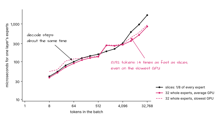
Up to 512 tokens, the two solid lines in Figure 9 stay within about 15% of each other, with the whole experts faster. The 12 replayed decode steps agree: the slices take 113 microseconds on average and the whole experts 102. Between 1,024 and 2,048 tokens, where neither a 64-request step nor an 8,192-token chunk falls, the whole experts are slower. Section 6 returns to the right half of the figure.

5.2 The Communication#

What the options send does differ. To see what that costs, I timed the two communication steps of a layer in isolation on all 8 GPUs: the all-gather and reduce-scatter of options 1 to 3, and FlashInfer’s dispatch and combine. The rows had 6,144 16-bit numbers, and I used the captured picks. Figure 10 shows the total time of each pair.

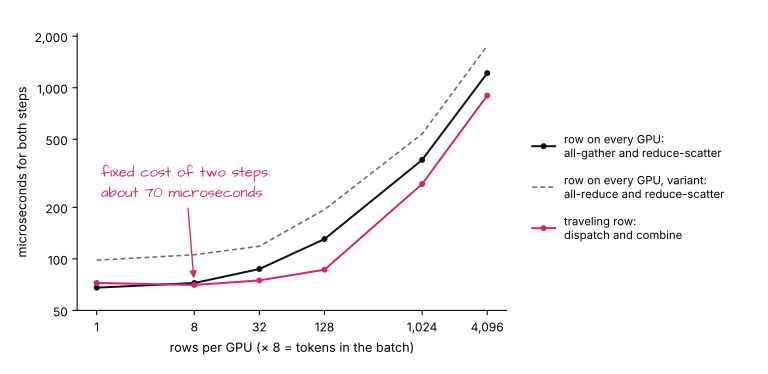
With 8 rows per GPU (a 64-token step), the two pairs take nearly the same time: 72 microseconds for the all-gather and reduce-scatter and 70 for dispatch and combine. A traveling row is sent to fewer GPUs, but even with 7 copies each, 64 rows are only 5.5 MB. We see the fixed cost of two steps that all 8 GPUs must synchronize on. For comparison, the expert kernel takes 102 to 113 microseconds.

Traveling rows are clearly faster only with more rows: 75 against 87 microseconds for 32 rows per GPU, and 86 against 131 for 128 rows.

5.3 The Server#

I ran GLM-5.3 as a server on all 8 GPUs with DP attention and changed one thing per configuration. The dense layers stayed sliced in all five configurations. Configurations 1 and 2 are options 1 and 2, configuration 3 is option 2 with one change, and configurations 4 and 5 are option 4. Configuration 3 is not option 3.

1. Slices: --tp-size 8 --attn-dp-size 8.
2. Whole experts with the row on every GPU: configuration 1 plus --ep-size 8.
3. The same with a copy of the shared expert on every GPU: configuration 2 plus the environment variable SGLANG_SHARED_EXPERT_TP1=1.
4. Traveling rows in 16 bits: configuration 1 plus --moe-a2a-backend flashinfer --moe-runner-backend flashinfer_trtllm_routed --flashinfer-a2a-dispatch-type bf16. The backend sets --ep-size 8 and copies the shared expert automatically, so apart from the entry point, the only change from configuration 3 is that the rows travel. The second flag selects the entry point from section 4.3.
5. Traveling rows in 4 bits: configuration 4 without --flashinfer-a2a-dispatch-type.

The load was ShareGPT text with 1,000 input tokens and 150 output tokens per request. I report the median time between consecutive tokens of a request (the inter-token latency), which is the time of one decode step. Figure 11 shows the results for 8, 64, and 256 concurrent requests.

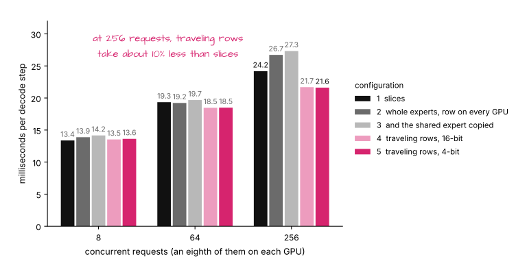
At 8 and 64 concurrent requests, all five configurations are within 7% of each other. With 8 requests, a step takes between 13.4 milliseconds for slices and 14.2 for configuration 3, with traveling rows 1% to 2% behind slices. At 64, they lie between 18.5 for traveling rows and 19.7 for configuration 3. Slices take 19.3 milliseconds at 64. By my one-layer estimate, the experts account for about 8.5 of that and the communication (75 layers × 72 microseconds) for about 5.4. The remaining 5.5 milliseconds are attention and everything else, which I didn’t break down.

At 256 concurrent requests, the configurations diverge. Slices take 24.2 milliseconds per step, whole experts with the row on every GPU take 26.7 (27.3 with the shared expert copied), and traveling rows take 21.7. A step with 256 tokens touches nearly every expert and gives each GPU 32 rows to send, which is where Figure 10 starts to favor traveling rows. Of the 2.5 milliseconds between slices and traveling rows, Figure 10 accounts for about 0.9 milliseconds. I can’t attribute the rest or explain why configuration 2 is slower than slices. Whether the rows travel as 16-bit or 4-bit values makes no measurable difference in a decode step: 21.7 against 21.6 milliseconds.

Configuration 3 is slower than configuration 2 at every load. With the row on every GPU, each GPU runs its whole copy of the shared expert for all rows of the batch, whereas in configuration 2, each GPU runs an eighth of it. The copy pays off only with traveling rows.

5.4 The Skew#

Whole experts give the GPUs unequal work. Figure 12 shows what the router does in one layer and what that means for 8 GPUs in one decode step.

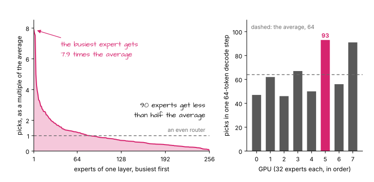
In the layer of Figure 12, the busiest expert gets 7.9 times the average, and 90 of the 256 experts get less than half of it. Across the 75 MoE layers, the busiest expert gets between 2.9 and 14 times the average. The 512 picks of a step are 64 per GPU on average, but in the step on the right, one GPU gets 93. SGLang reports this as balancedness, the average picks per GPU divided by the busiest GPU’s picks (simplified from here):

# picks_per_gpu: (layers, gpus)
picks = picks_per_gpu.float()
balancedness = picks.mean(dim=-1) / picks.max(dim=-1).values

For this step, that’s 64 / 93 = 0.69. Averaged over all 300 steps and all layers, it’s 0.75.

A balancedness of 0.75 suggests that the GPUs idle a quarter of the time. That would be true only if a GPU’s time followed its picks, but section 2 showed that the time follows the bytes read. A calculation with the line from Figure 4 shows the difference. At 21 MB per expert, a GPU that gets 100 picks on 12 experts reads about 255 MB and takes 66 microseconds. A GPU that gets 50 picks on 28 experts reads about 595 MB and takes 117. That’s twice the picks and a little more than half the time.

In the 12 replayed steps, the GPU with the most picks got between 75 and 114, against an average of 63 (63 tokens × 8 picks / 8 GPUs). It was the slowest GPU in only one step. In all 12 steps, the slowest GPU was among those that read the most expert weights. No GPU can read more than its 32 experts, which caps the spread. The slowest whole-expert GPU took 113.7 microseconds against 102.1 for the average one, 11% more, not the 33% that 1 / 0.75 suggests.

The server runs agree. SGLang has a switch for benchmarks, SGLANG_SIMULATE_ROUND_ROBIN_EXPERTS=1, that overwrites the router’s picks with a round-robin assignment. Every GPU then gets the same number of picks, and every row gets one expert on each of the 8 GPUs. I ran configuration 5 with it. At 64 concurrent requests, a decode step takes 19.8 milliseconds instead of 18.5, so perfect balance is 7% slower. The round-robin assignment touches all 256 experts, whereas the router touches 72%, and it sends 7 copies of every row instead of 4.6. The switch changes these along with the balance, and I can’t separate them. At 8 and 256 concurrent requests, the two are within 2% of each other.

A common remedy for uneven load is the Expert Parallelism Load Balancer (EPLB) from DeepSeek, which SGLang enables with --enable-eplb. It records how many picks each expert gets, copies popular experts into spare slots, and places all slots so that the GPUs’ loads are as even as possible. I ran my own copy of SGLang’s algorithm on the first half of my recorded decode steps and scored the placement on the second half. With 32 spare slots per layer, 4 per GPU, the balancedness on 8 GPUs rises from 0.75 to 0.86. The placement slightly exceeds an even router, which reaches 0.85 with 512 picks per step, and what remains is chance.

But EPLB balances picks, and in a decode step, time doesn’t follow picks. At most, a better placement could bring the slowest GPU down to the average, a gain of about 10% of that GPU’s kernel time. The copies of popular experts add bytes to read. I didn’t measure a server with EPLB, so this is an inference from section 2.

To summarize, in a decode step on 8 GPUs with up to 64 concurrent requests, how a row meets its experts hardly matters, because every option reads the same bytes and pays the same fixed cost to communicate. Is that also true for a prefill chunk?

6. Prefill on 8 GPUs#

A prefill chunk lies at the right end of Figure 3. With 8,192 tokens, every expert is touched many times over, the arithmetic dominates, and by the rule from section 2, we count rows.

6.1 The Kernel#

The right half of Figure 9 shows the kernel times for prefill-sized batches. For a chunk of 8,192 tokens, an eighth of every expert takes 609 microseconds, whereas 32 whole experts take 353 microseconds on average and 432 on the slowest of the 8 GPUs. At 32,768 tokens, the largest batch I replayed, slices take 1,707 microseconds and whole experts 852 on average.

These numbers are for a kernel tuned by FlashInfer’s autotuner, which tries several internal settings per batch size and keeps the fastest. By default, SGLang with DP attention tunes only decode-sized batches, and SGLANG_FLASHINFER_AUTOTUNE_EXTEND=1 extends the tuning to prefill-sized batches. Untuned, the 8,192-token chunk takes 1,017 microseconds for slices and 821 for the slowest whole-expert GPU. On the slowest GPU, whole experts are 1.4 times as fast when tuned and 1.2 times when untuned.

6.2 The Communication#

Figure 10 also covers prefill-sized batches. With 1,024 rows per GPU (an 8,192-token chunk), the all-gather and reduce-scatter take 379 microseconds per layer, and dispatch and combine take 274. With 4,096 rows per GPU, the times are 1,217 against 900 microseconds. The ratio of about 1.4 is a little below the ratio of the copies, 7 against 4.6.

SGLang records the kernels of a prefill chunk once and replays them as one unit, the prefill CUDA graph. For prefill batches that run outside this graph, it replaces the all-gather with an all-reduce, a collective that sums a buffer over all GPUs and gives every GPU the sum. In the same test, the pair with the all-reduce takes 538 microseconds for 1,024 rows per GPU, twice as long as dispatch and combine. My servers rarely used this variant: configurations 1 to 3 ran over 95% of their chunks inside the graph, which keeps the all-gather.

For an 8,192-token chunk, a layer with slices and a tuned kernel spends about 60% as long moving rows as it spends on the experts.

6.3 The Server#

For prefill, I sent prompts of 8,000 tokens, 16 at a time, to the same five configurations and measured input tokens per second. The prefill kernel was untuned, the default. Figure 13 shows the results and two runs that used the tuned prefill kernel.

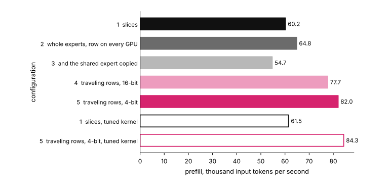
Slices reach 60,200 input tokens per second, and whole experts with the row on every GPU reach 64,800. Traveling rows reach 77,700 in 16 bits and 82,000 in 4 bits. The last configuration processes prompts 1.36 times as fast as the first, and most of the gain comes from letting the rows travel. Configuration 3, which copies the shared expert without traveling rows, is again the slowest at 54,700.

With the tuning switched on, slices reach 61,500 tokens per second and traveling 4-bit rows 84,300. That is a gain of 2% to 3%, which is smaller than the 3% to 6% by which my two runs of each configuration differ. I confirmed in the logs that the tuned servers tuned the 8,192-token size and that the untuned ones did not reuse that result.

In the replay, tuning saves slices 408 microseconds per layer (1,017 minus 609), or about 31 milliseconds over 75 layers. At 60,200 tokens per second, the server spends about 136 milliseconds on a chunk, and 31 is over a fifth of that. On the server, tuning saved less than in the replay. I haven’t compared the settings that the two chose.

6.4 The Skew in Prefill#

With the tuned kernel, a GPU’s prefill time rises with its picks, but less than proportionally. For the one replayed 8,192-token chunk, the GPU with the most picks got 13,892, against an average of 8,192 (8 picks per token over 8 GPUs). Its kernel took 432 microseconds against 353 for the average GPU. That’s 1.7 times the picks and 1.2 times the time. With the untuned kernel, which my servers ran, the same GPU takes 747 microseconds, the same as the average of the 8, and the slowest GPU is one with few picks. In both cases, the other 7 GPUs wait for the slowest one.

On the server, the round-robin switch changes nothing for prefill: configuration 5 reaches 81,900 tokens per second with it and 82,000 without. The switch balances the picks, but it also sends 7 copies per row instead of 4.6, so I can’t separate the two effects.

The balancedness of my recorded prefill batches is 0.79 on 8 GPUs, and EPLB’s placement brings it to 0.89. An even router would reach 0.99. These are counts of picks, not times, from only the 5 of 9 prefill batches on which I scored the placement.

6.5 Two Ways to Overlap the Communication#

SGLang has two mechanisms that overlap communication with computation.

The first is a fused kernel. In the configurations above, dispatch, the experts, and combine run as three kernels, one after the other. A fused kernel does all three, so a GPU can start on the first rows that arrive while later rows are still in transit. SGLang selects one with --moe-a2a-backend megamoe or flashinfer_megamoe. I ran flashinfer_megamoe once on GLM-5.3, but SGLang disabled the prefill CUDA graph for this backend. I couldn’t confirm that I had configured it as intended, so I don’t report the run.

The second is two-batch overlap (--enable-two-batch-overlap). It splits a batch in two and interleaves the halves so that one half runs its attention or its experts while the other half’s rows are in transit. I didn’t measure it.

6.6 Separate Prefill and Decode Servers#

With prefill and decode on separate servers, the disaggregated serving from the introduction, each can get the option that suits it. On 8 GPUs, however, traveling rows are the fastest option for prefill and, from 64 concurrent requests on, for decoding. Separate servers also allow the fifth option: only on a prefill server can a GPU’s computation take longer than DWDP’s weight copies.

To summarize, in a prefill chunk on 8 GPUs, whole experts are faster in the kernel, and traveling rows are faster in the communication. A server that combines them processes prompts 1.36 times as fast as one with slices. Balance matters only where time follows picks, which it does not in a decode step. In prefill, the slowest GPU’s tuned kernel took 1.2 times the average in the one chunk that I replayed.

So far, everything has been for 8 GPUs. What changes when there are more?

7. Beyond 8 GPUs: A Calculation#

Rack systems connect far more than 8 GPUs directly, and published recipes for them use up to 48 GPUs per server. Nothing in this section is measured: it is arithmetic on the model’s dimensions and on my recorded picks, which I regroup as if the same 256 experts were spread over more GPUs.

With slices, and with any option that puts the row on every GPU, a row is sent to N − 1 GPUs, so to 31 GPUs when N is 32. A traveling row is sent to the GPUs that hold its experts, and since a row has only 8 experts, it never needs more than 8 copies. The left side of Figure 14 shows the two curves.

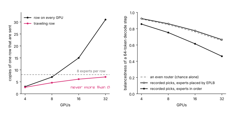
The traveling row’s curve comes from the formula of section 4.3, minus the row’s own GPU, which gives 6.1 copies on 16 GPUs and 7.0 on 32.

A slice also gets narrower: 128 numbers wide on 16 GPUs and 64 on 32. The kernel that I measured needs the width to be a multiple of 128, so SGLang pads narrower slices to 128. If the number of GPUs doesn’t divide 2,048 evenly, as with 24 or 48, a server with slices fails at startup. Whole experts keep their full width on any number of GPUs.

For a decode step, we count the bytes that each GPU reads. The rule from section 2 applies directly, because the experts that a step touches don’t depend on the number of GPUs. A step of the replayed layer touches about 188 experts, which is 4.0 GB with scale factors, whether the experts are spread over 8 GPUs or 32.

Per GPU, that’s 0.50 GB on 8 GPUs and 0.125 GB on 32, which is below the range that I fitted. If the line from Figure 4 held there, a GPU’s expert kernel would take 28 + 150 × 0.125 = 47 microseconds per layer on 32 GPUs, where I measured 102 on 8. More GPUs therefore mean less reading per GPU, but the communication does not shrink if the fixed cost of Figure 10 holds on more GPUs, because every layer still needs dispatch and combine.

The balancedness gets worse, as the right side of Figure 14 shows. With the experts in their original order, the balancedness of a 64-token step falls from 0.75 on 8 GPUs to 0.61 on 16 and 0.46 on 32. EPLB’s placement brings it to 0.78 on 16 and 0.67 on 32, slightly above an even router’s 0.76 and 0.65, as on 8 GPUs. What remains is the randomness of 512 picks spread over that many GPUs. These are counts of picks, and for a decode step, section 5.4 showed that time doesn’t follow picks. I have no measurement of what a balancedness of 0.46 costs on 32 GPUs.

For prefill, time rises with the picks (section 6.4, tuned kernel), and the counts show a clearer trend. In 5 of my 9 recorded prefill batches, the balancedness with the original order is 0.79 on 8 GPUs, 0.66 on 16, and 0.51 on 32, whereas an even router would reach 0.99, 0.97, and 0.96.

The SGLang post on EPLB reports that EPLB made prefill 1.49 times and decoding 2.54 times as fast for DeepSeek-V3 on a cluster of 96 H100 GPUs. Its placement was computed from the same data that it was then tested on. By its reported throughput and latency, that deployment decoded several hundred rows per expert in a step. That is the part of Figure 3 where time follows rows, so it doesn’t contradict my 64-token steps.

In InferenceX, SemiAnalysis’s inference benchmark, the largest DeepSeek-R1 decode servers on GB200 racks have 24 to 48 GPUs and use whole experts with traveling rows. The prefill servers paired with them use 8 GPUs with traveling rows or 4 GPUs with slices. These recipes use DeepEP, a different all-to-all backend from the one I measured, and they copy the dense layers. Balancing is rare: of the 119 SGLang recipes for four MoE model families in that benchmark, one turns EPLB on.

To summarize the calculation: with more GPUs, traveling rows never need more than 8 copies and keep their experts whole, every GPU reads less, and the balancedness of the picks gets worse.

8. How I Measured and What I Left Out#

All measurements ran on one machine with 8 B300 GPUs, with SGLang at commit f1065423 and FlashInfer 0.7.0.post1, on the NVFP4 checkpoint of GLM-5.3.

The picks come from SGLang’s recorder, which counts, for every forward pass (one decode step or one prefill batch), how many picks each expert of each layer gets. I ran it on a server with 2 GPUs under 128 requests of ShareGPT text with 1,000 input and 150 output tokens, 64 at a time. I used the 300 decode steps with exactly 64 tokens and the 9 prefill batches, which hold about 14,000 tokens each. The picks of a row don’t depend on the number of GPUs, so regrouping them for 8 GPUs is exact.

The kernel times come from a separate server run. For one MoE layer (the 37th of 75), I captured the expert weights, the input rows, and the picks, for prefill chunks and for 120 consecutive decode steps of 63 tokens, of which I replayed the first 12 one by one. Decode batches of other sizes in Figure 3 are the first rows of these steps, joined end to end. I replayed them on one B300 through the same FlashInfer kernel that SGLang calls, first with an eighth of every expert, then with each of the 8 groups of 32 whole experts. The times come from CUPTI, CUDA’s profiling interface, and each is the median of three runs. Unless I say otherwise, as in sections 6.1 and 6.4, the kernel is tuned for each batch size.

For Figure 10, I ran the two communication steps on all 8 GPUs outside a server, with random 16-bit rows of GLM-5.3’s size and the picks from the kernel capture. An iteration takes as long as its slowest GPU, measured between two CUDA events on that GPU, and I report the median of three runs, each the median of 30 iterations. The expert kernel doesn’t run in between, so these times don’t include contention with it. On the server, these steps run inside a CUDA graph between other kernels, and prefill pads every GPU to a shared size.

Every 8-GPU server except section 3’s tensor-parallel one ran with DP attention, --chunked-prefill-size 8192 (1,024 tokens per GPU), at most 256 concurrent requests, and no speculative decoding. For decoding, the load was ShareGPT text with 1,000 input and 150 output tokens. For prefill, it was 8,000 input tokens with 1 output token, 16 requests at a time, and an empty prefix cache. Each server number is the mean of two repetitions, which differ by less than 1% for decoding and by up to 6% for prefill.

I replayed only one layer of 75 and measured one model, one weight format, and one kernel family. In the server runs, I changed one thing per configuration, but a flag can change more than the MoE layer, and I can’t separate those effects.

I left out:

• How dispatch and combine are implemented in the different backends, and the fused kernels beyond section 6.5
• The router’s matrix product
• DP attention beyond section 3
• Elastic expert parallelism, where GPUs join or leave the expert group while the server runs
• Running some experts on the CPU
• Model-specific flags: --moe-dp-size, which belongs to context parallelism for Qwen3 MoE models, and the flags that slice the shared expert of Kimi K3 within a subgroup of GPUs

9. Summary#

To wrap up, Figure 15 collects the answers.

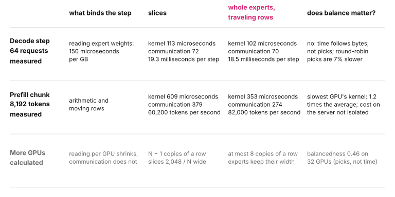
In a decode step, the experts’ time is bound by reading their weights. On 8 GPUs, the measured options read the same bytes, the communication costs about 70 microseconds per layer at 64 concurrent requests either way, and the servers are within 7% of each other up to that load. At 256 concurrent requests, traveling rows take about 10% less time than slices. Round-robin picks touch every expert and are 7% slower at 64 requests.

A prefill chunk spends its time on arithmetic and on moving rows. There, whole experts are 1.4 times as fast in a tuned kernel, even on the slowest GPU, and dispatch and combine are 1.4 times as fast as the all-gather and reduce-scatter. The server with traveling 4-bit rows processes prompts 1.36 times as fast as the server with slices.

Beyond 8 GPUs, the calculation says that a traveling row never needs more than 8 copies, whereas the copies in options 1 to 3 grow with the number of GPUs. It also says that the reading per GPU shrinks while every layer still needs dispatch and combine.

Coming back to the question from the beginning: for GLM-5.3 in NVFP4 on 8 B300 GPUs, with FlashInfer’s backend and no speculative decoding, a row should travel to its experts. In a decode step, that costs 1% to 2% at 8 concurrent requests and saves about 10% at 256, and in prefill, it gains 36%.